Ingeotec at DA-VINCIS: Bag-of-Words Classifiers

IberLEF 2023, September 2023, Jaén, Spain

Mario Graff

INFOTEC

Daniela Moctezuma

CentroGEO

Eric S. Téllez

INFOTEC

Sabino Miranda-Jiménez

INFOTEC

INGEOTEC research group

GitHub: https://github.com/INGEOTEC
WebPage: https://ingeotec.github.io/

Introduction

Violence is a serious problem that can have a devastating impact on individuals and communities.

In some cases, the virtual world is prone to aggressive expressions and insults, among other violent expressions.

The DA-VINCIS Task at IberLEF 2023

An open challenge to develop multimodal models to detect violent incidents on Twitter. The task has two tracks:

1. violent event identification and
2. violent event category recognition.

This presentation describes our solution system for the (i) track using only text-based features. More particularly, we used our EvoMSA framework (Graff et al. 2020).

Our appproach

Since we focus on text messages, violent event identification can be seen as a text classification task.

Given the content of a tweet written in natural language, our model must identify whenever a violent event is mentioned.

Our approach: EvoMSA 2.0

Our representations

• Sparse bag of words (SBOW)
• Dense bag of words (DBOW)

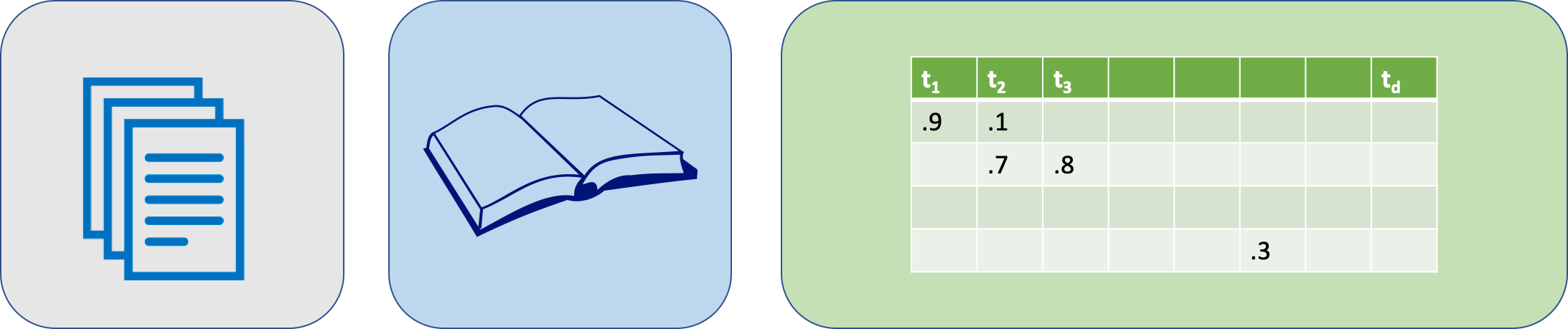
Sparse bag of words

The text is preprocessed and tokenized, then each token \(t\) is associated with a vector \(\mathbf{v_t} \in \mathbb R^d\) where the \(i\)-th component, i.e., \(\mathbf{v_t}_i\), contains the Inverse-Document-Frequency (IDF) value of the token \(t\) and \(\forall_{j \neq i} \mathbf{v_t}_j=0\).

The set of vectors \(\mathbf V = \{ \mathbf v_t \}\) corresponds to the vocabulary, and there are \(|\mathbf V| = d\) different tokens in the vocabulary.

A text is represented by the sequence of its tokens, i.e., \((t_1, t_2, \ldots)\). The text is then vectorized as:

\[ \textsf{sbow}(\text{some text}) = \textsf{sbow}((t_1, t_2, \ldots)) = \frac{\sum_t \mathbf{v_t}}{\lVert \sum_t \mathbf{v_t} \rVert} \]

SBoW

Dense bag of words

In contrast to SBOW, the dense embeddings come from associating each component to the decision value of a text classifier (e.g., based on SBOW) pre-trained on a different collection of tweets.

Without loss of generality, it is assumed that there are \(M\) labeled datasets, each one contains a binary text classification problem.

noting that if a dataset has \(K\) labels, then this dataset can be represented as \(K\) binary classification problems following the one versus the rest approach, i.e., it is transformed to \(K\) datasets.

Construction of the DBOW

For each of these \(M\) binary text classification problems, a SBOW-based classifier is built using a pre-trained SBOW representation and a linear Support Vector Machine (SVM) as the classifier. Consequently, there are \(M\) binary text classifiers, i.e., \((c_1, c_2, \ldots, c_M)\). Additionally, the decision function of \(c_i\) is a value where the sign indicates the class.

The text representation is the vector obtained by concatenating the decision functions of the \(M\) classifiers and then normalizing the vector to have unitary norm.

Construction (continued…)

A text \(x\) is represented with vector \(\mathbf{x^{'}} \in \mathbb R^M\) where the value \(\mathbf{x^{'}}_i\) corresponds to the decision function of \(c_i\). Given that the classifier \(c_i\) is a linear SVM, the decision function corresponds to the dot product between the input vector and the weight vector \(\mathbf w_i\) plus the bias \(\mathbf w_{i_0}\), where the weight vector and the bias are the parameters of the classifier.

Construction (continued…)

That is, the value \(\mathbf{x^{'}}_i\) corresponds to

\[ \mathbf{x^{'}}_i = \mathbf w_i \cdot \frac{\sum_t \mathbf{v_t}}{\lVert \sum_k \mathbf{v_k} \rVert} + \mathbf w_{i_0}, \]

where \(\mathbf{v_t}\) is the IDF vector associated to the token \(t\) of the text \(x\)

Construction (continued…)

In matrix notation, vector \(\mathbf{x'}\) is

\[ \mathbf{x^{'}} = \mathbf W \cdot \frac{\sum_t \mathbf{v_t}}{\lVert \sum_k \mathbf{v_k} \rVert} + \mathbf{w_0}, \]

where matrix \(\mathbf W \in \mathbb R^{M \times d}\) contains the weights, and \(\mathbf{w_0} \in \mathbb R^M\) is the bias. Another way to see the previous formulation is by defining a vector \(\mathbf{u_t} = \frac{1}{\lVert \mathbf{v_t} \rVert} \mathbf W \mathbf{v_t}\).

Construction (continued…)

Consequently, \(\mathbf{x'}\) is defined as:

\[ \label{eq:denseBoW} \mathbf{x'} = \sum_t \mathbf{u_t} + \mathbf{w_0}, \] vectors \(\mathbf{u} \in \mathbb R^M\) correspond to the tokens. This is the reason we refer to this model as a dense BoW.

Finally, the vector representing the text \(x\) is the normalized \(\mathbf{x^{'}}\), i.e., \(\mathbf x = \frac{\mathbf{x^{'}}}{\lVert \mathbf{x^{'}} \rVert}.\)

Dense BoW (stacking)

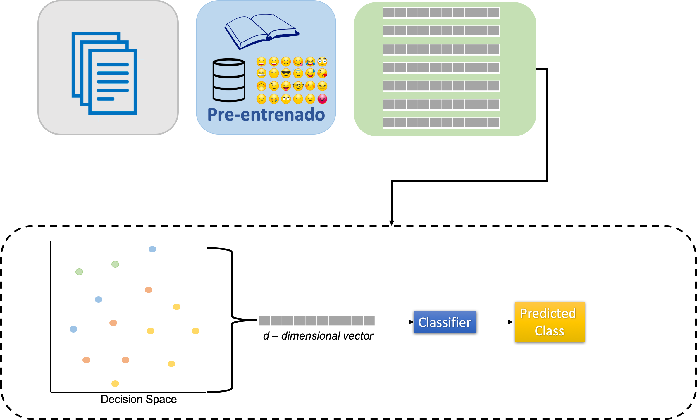
Stacking: All models aggregated are used according to their weights for producing an output, the final classification.

SBOW parameters

Different BoW representations were created and implemented following the approach described in (Tellez et al. 2017). The first step was to set all the characters to lowercase and remove diacritics and punctuation symbols. Additionally, the users and the URLs were removed from the text. Once the text is normalized, it is split into bigrams, words, and q-grams of characters with \(q=\{2, 3, 4\}.\)

SBOW parameters (continued…)

The pre-trained BoW is estimated from 4,194,304 (\(2^{22}\)) tweets randomly selected in a larger collection of messages.

The IDF values were estimated from the collections, and some tokens were selected from all the available ones found in the collection.

SBOW parameters (continued…)

Two procedures were used to select the tokens:

1. the first corresponds to selecting the \(d\) tokens with the highest frequency, and the other to normalize the frequency w.r.t. their type, i.e., bigrams, words, and q-grams of characters. Once the frequency is normalized, one selects the \(d\) tokens with the highest normalized frequency.
2. The value of \(d\) is \(2^{17}\); however, one can also find in the library models for \(2^{13}, 2^{14}, \ldots, 2^{17}.\)

SBOW parameters (continued…)

It is also possible to train the BoW model using the training set; in this case, we used the default parameters. The only difference is that vocabulary size \(d\) is bounded by the training set tokens.

DBOW parameters

The dense representations start by defining the labeled datasets used to create them. These datasets are organized in three groups.

1. A set human-annotated datasets; we refer to them as dataset.
2. A set of self-supervised dataset where the objective is to predict the presence of an emoji as expected; these models are referred to as emoji.
3. A set of self-supervised datasets where the task is to predict the presence of a particular word, namely keyword.

The keyword group includes a set of dense representations where the words were selected from the training set; we refer to these representations as tailored.

The words were the most discriminative based on the BoW classifier; these were the ones with the highest absolute value between the product of the coefficient computed by the linear SVM and the IDF coefficient.

DBOW parameters (continued…)

Following an equivalent approach used in the development of the pre-trained BoW, different dense representations were created.

These correspond to varying the size of the vocabulary and the two procedures used to select the tokens. Vector spaces:

• dataset is in \(\mathbb R^{57}\).
• emoji is in \(\mathbb R^{567}\).
• keyword is in \(\mathbb R^{2048}\).

Configurations

We tested 13 different algorithms for each task. The configuration having the best performance was submitted to the contest. The best performance was computed using k-fold cross-validation (\(k=5\)).

Configurations (continued…)

The different configurations tested in this competition are described below. These configurations include BoW and a combination of BoW with dense representations. Stack generalization combines the different text classifiers, and the top classifier was a Naive Bayes algorithm. The specific implementation of this configuration can be seen in EvoMSA’s documentation.

Configurations (continued…)

The list of configurations

• bow: Pre-trained BoW where the tokens are selected based on a normalized frequency w.r.t. its type, i.e., bigrams, words, and q-grams of characters.
• bow_voc_selection: Pre-trained BoW where the tokens correspond to the most frequent ones.
• bow_training_set: BoW trained with the training set; the number of tokens corresponds to all the tokens in the set.
• stack_bow_keywords_emojis: Stack generalization approach where the base classifiers are the BoW, the emojis, and the keywords dense BoW.
  
• stack_bow_keywords_emojis_voc_selection: Stack generalization approach where the base classifiers are the BoW, the emojis, and the keywords dense BoW. The tokens in these models were selected based on a normalized frequency w.r.t. its type, i.e., bigrams, words, and q-grams of characters.

Configurations (continued…)

• stack_bows: Stack generalization approach where the base classifiers are BoW with the two token selection procedures described previously (i.e., bow and bow_voc_selection).
• stack_2_bow_keywords: Stack generalization approach where with four base classifiers. These correspond to two BoW and two dense BoW (emojis and keywords), where the difference in each is the procedure used to select the tokens, i.e., the most frequent or normalized frequency.
• stack_2_bow_tailored_keywords: Stack generalization approach with four base classifiers. These correspond to two BoW and two dense BoW (emojis and keywords), where the difference in each is the procedure used to select the tokens, i.e., the most frequent or normalized frequency. The second difference is that the dense representation with normalized frequency also includes models for the most discriminant words selected by a BoW classifier in the training set. We refer to these latter representations as tailored keywords.

Configurations (continued…)

• stack_2_bow_all_keywords: Stack generalization approach with four base classifiers equivalent to stack_2_bow_keywords where the difference is that the dense representations include the models created with the human-annotated datasets.
• stack_2_bow_tailored_all_keywords: Stack generalization approach with four base classifiers equivalent to stack_2_bow_all_keywords, where the difference is that the dense representation with normalized frequency also includes the tailored keywords.
• stack_3_bows: Stack generalization approach with three base classifiers. All of them are BoW; the first two correspond pre-trained BoW with the two token selection procedures described previously (i.e., bow and bow_voc_selection), and the latest is a BoW trained on the training set (i.e., bow_training_set).

Configurations (continued…)

• stack_3_bows_tailored_keywords: Stack generalization approach with five base classifiers. The first corresponds to a BoW trained on the training set, and the rest are used in stack_2_bow_tailored_keywords.
• stack_3_bow_tailored_all_keywords: Stack generalization approach with five base classifiers. It is comparable to stack_3_bows_tailored_keywords being the difference in the use of the tailored keywords.

Results

Configuration	Tailored	Dense	DA-VINCIS 2023	DA-VINCIS 2022
stack_2_bow_tailored_all_keywords	X	X	0.8984	0.8361
stack_2_bow_all_keywords		X	0.8951	0.8447
stack_3_bows_tailored_keywords	X	X	0.8971	0.7555
stack_3_bow_tailored_all_keywords	X	X	0.8968	0.8219
stack_2_bow_tailored_keywords	X	X	0.8966	0.7572
stack_2_bow_keywords		X	0.8955	0.7525
stack_3_bows	X		0.8931	0.7329
bow_voc_selection			0.8907	0.7342
bow			0.8894	0.7324
bow_training_set	X		0.8892	0.7337
stack_bows			0.8879	0.7329
stack_bow_keywords_emojis		X	0.8863	0.7595
stack_bow_keywords_emojis_voc_selection		X	0.8859	0.7588

Performance, in terms of F1, of different configurations on a five fold cross-validation. The best performance is in boldface.

The Table presents the performance, in terms of F1, of the different configurations in the k-fold cross-validation (\(k=5\)). It also includes the performance of our submission in the competition and the competition’s winner. The table includes two columns Tailored and Dense; these provide an overview of the systems. The tailored column indicates whether the training set was used to define the words in the self-supervised datasets or the BoW vocabulary was obtained from it. The dense column indicates the use of a dense representation.

It can be observed that, for edition 2023, the best configuration is a stack generalization algorithm with four base classifiers; two BoW and two dense representations. One of the dense models also includes tailored keywords. The best configuration for edition 2022 is quite similar to the one for 2023; the difference is that the 2022 configuration does not use tailored keywords. The configuration used in 2023 is the second-best configuration of 2022, according to the performance obtained in the k-fold cross-validation approach.

Competition

Performance comparison of our submission (INGEOTEC) and the competition’s winner in each edition. The best performance is in boldface.

	DA-VINCIS 2023	DA-VINCIS 20222
Winner	0.9264	0.7817
INGEOTEC	0.8903	0.7510
Difference	4.1%	4.1%

Another comparison that one can make with the Table’s data is computing the difference between the best performance in k-fold cross-validation and the worst; it can be observed that for the 2023 edition, the difference is 1.4%, and for 2022 is 13.3%. The difference of 1.4% indicates that following this approach will be complicated to improve. On the other hand, for the edition 2022, there might be room for improvement following the presented approach.

Other competitions performance

Performance comparison. EvoMSA’ results

Competition	Winner	EvoMSA 2.0	Difference
PoliticEs (Gender)	0.8296	0.7115	16.6%
PoliticEs (Profession)	0.8608	0.8379	2.7%
PoliticEs (Ideology Binary)	0.8967	0.8913	0.6%
PoliticEs (Ideology Multiclass)	0.6913	0.6694	3.3%
REST-MEX (Polarity)	0.6216	0.5548	12.0%
REST-MEX (Type)	0.9903	0.9805	1.0%
REST-MEX (Country)	0.9420	0.9270	1.6%

Other competitions performance (Continued…)

Performance comparison. EvoMSA’ results

Competition	Winner	EvoMSA 2.0	Difference
HOMO-MEX	0.8847	0.8050	9.9%
HOPE (ES)	0.9161	0.4198	118.2%
HOPE (EN)	0.5012	0.4429	13.2%
DIPROMATS (ES)	0.8089	0.7485	8.1%
DIPROMATS (EN)	0.8090	0.7255	11.5%
HUHU	0.820	0.775	5.8%

Example

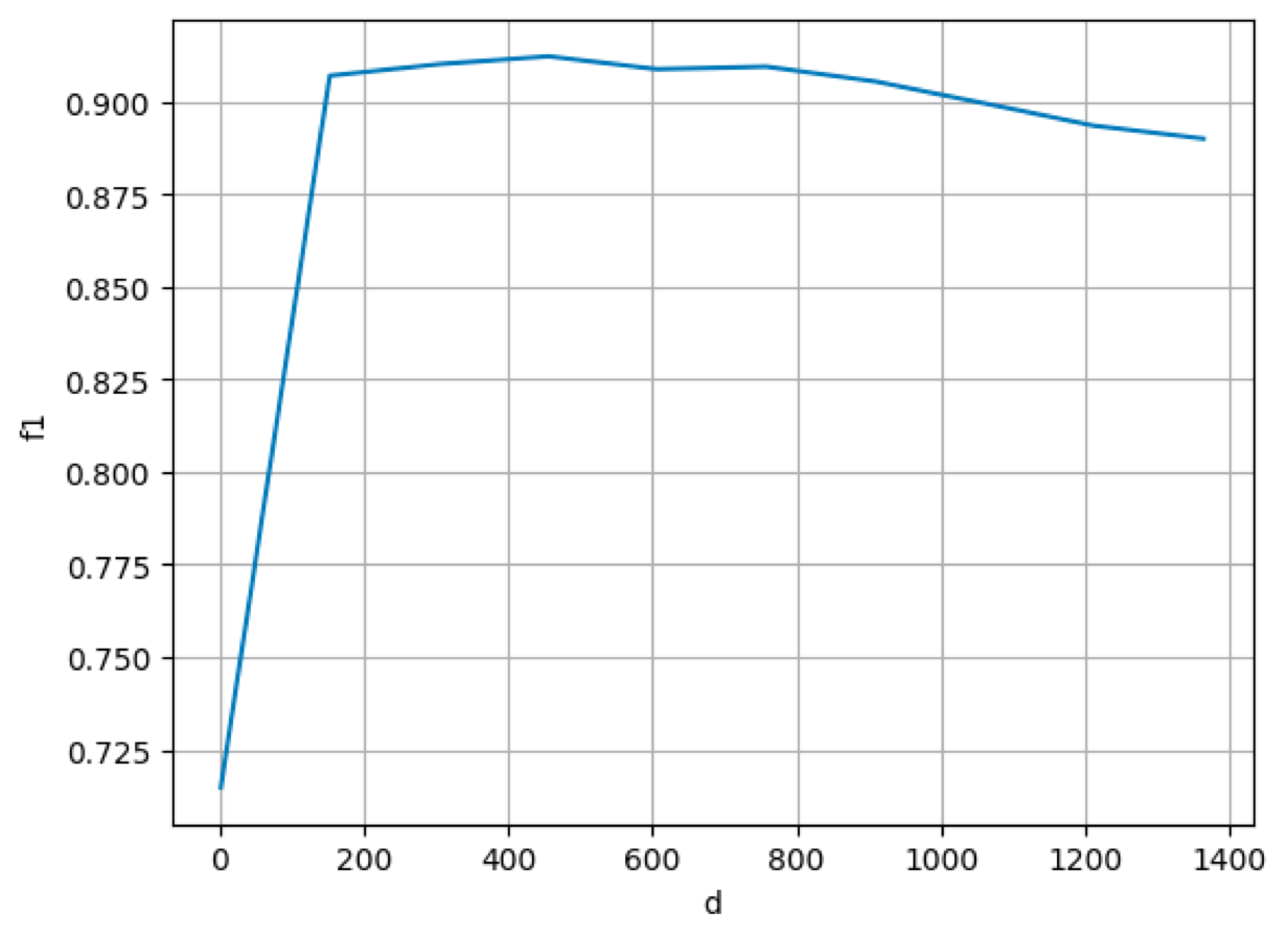
Using a tailored dense model with the DA-VINCIS 2023 dataset, we can see:

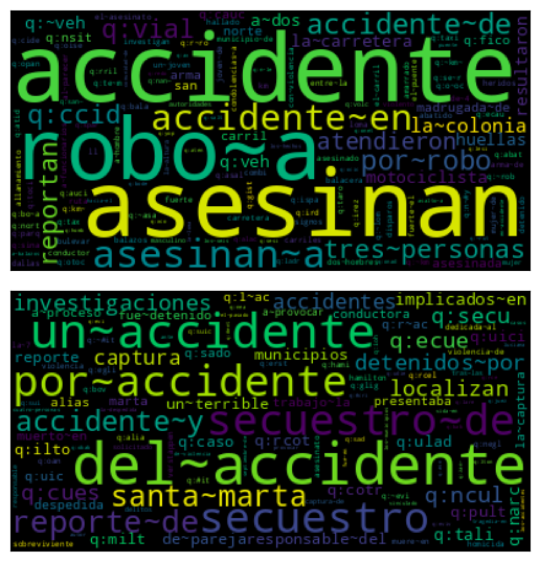
Example - performance varying \(d\)

Conclusions

We have presented our system solution and results for detecting violent incidents on Twitter using only text-based features in the context of the DA-VINCIS 2023 challenge.

• Our system is based on the ensemble of multiple models using stacked generalization, more precisely with our EvoMSA framework.
• Our approach uses lexical and semantic features, all computed as bags of words.
• We achieved an F1 score of 0.89, just 3 hundredths behind the best model in the final ranking.
• Our results show that developing competitive models for violent event identification is possible using only text-based features and, even more, bag-of-words-based models.

This is important when: - it is impossible to afford the prediction costs of transformer-based solutions. - some degree of explainability is required, we can always retrieve the words involved in the decision model

Conclusions (continued…)

Explainability of the model (with a simple bow outstanding results). Simplest solution Fast solution (in training and test), low computational resources. Dense representation using at most 100 million tweets.

Thanks

Questions?

Also, we want to promote the usage of our EvoMSA library.

For EvoMSA documentation see:
https://evomsa.readthedocs.io/en/docs/
EvoMSA Github repository
https://github.com/INGEOTEC/EvoMSA

References

Graff, Mario, Sabino Miranda-Jimenez, Eric S Tellez, y Daniela Moctezuma. 2020. «Evomsa: A multilingual evolutionary approach for sentiment analysis [application notes]». IEEE Computational Intelligence Magazine 15 (1): 76-88.

Tellez, Eric S., Sabino Miranda-Jiménez, Mario Graff, Daniela Moctezuma, Ranyart R. Suárez, y Oscar S. Siordia. 2017. «A simple approach to multilingual polarity classification in Twitter». Pattern Recognition Letters 94: 68-74. https://doi.org/10.1016/j.patrec.2017.05.024.