Exploratory Data Analysis of Diario Oficial Titles, 1917–2026

A first exploration of the note archive

Published

July 17, 2026

Abstract

We examine the titles of the 1,232,802 notes published in Mexico’s Diario Oficial de la Federación between January 1917 and June 2026, obtained from the gazette’s own open-data service. Reading yearly volume, the first word of each title, title length, the issuing branch recorded on every note and the vocabulary that sets a year or a presidential term apart, the analysis reveals three major transformations: the expansion of the gazette from 1999 onward, when the systematic cataloguing of procurement announcements and notices doubled the number of notes; the displacement of the classic legal instruments — resoluciones and decretos — by the administrative aviso as the dominant documentary form; and the correlative impoverishment of the title as a descriptor, whose median length fell from about twenty words to five or six.

Open in Colab

Imports and the styling shared by every figure

from pathlib import Path

import matplotlib as mpl
import matplotlib.pyplot as plt
import pandas as pd
import plotly.graph_objects as go

# Validated categorical palette (light mode), in fixed assignment order.
BLUE, GREEN, MAGENTA, YELLOW = "#2a78d6", "#008300", "#e87ba4", "#eda100"
LIGHT_BLUE = "#9ec5f4"  # step 200 of the blue sequential ramp
INK, MUTED, GRID, AXIS = "#52514e", "#898781", "#e1e0d9", "#c3c2b7"

mpl.rcParams.update(
    {
        "figure.facecolor": "white",
        "axes.facecolor": "white",
        "axes.spines.top": False,
        "axes.spines.right": False,
        "axes.edgecolor": AXIS,
        "axes.labelcolor": INK,
        "axes.titlecolor": INK,
        "xtick.color": MUTED,
        "ytick.color": MUTED,
        "text.color": INK,
        "font.size": 10,
        "axes.axisbelow": True,
    }
)


def clean_axis(ax):
    ax.grid(axis="y", color=GRID, linewidth=0.8)
    ax.tick_params(length=0)
    ax.set_xlabel("")


def thousands(x, _):
    return f"{int(x):,}"


# Shared Plotly styling, mirroring the matplotlib figures' academic look: a white
# surface, a light horizontal grid only, no spines, muted ticks, ink-colored text
# and a unified hover box. Reused by every interactive figure on this page.
PLOTLY_FONT = "system-ui, -apple-system, 'Segoe UI', Helvetica, Arial, sans-serif"


def style_plotly(fig, *, yaxis_title="", height=430):
    fig.update_layout(
        font=dict(family=PLOTLY_FONT, size=13, color=INK),
        paper_bgcolor="white",
        plot_bgcolor="white",
        height=height,
        margin=dict(l=64, r=24, t=16, b=40),
        hovermode="x unified",
        hoverlabel=dict(bgcolor="white", bordercolor=GRID, font=dict(color=INK, size=12)),
        legend=dict(font=dict(size=12, color=INK)),
    )
    fig.update_xaxes(
        showgrid=False, showline=False, zeroline=False,
        ticks="", tickfont=dict(color=MUTED), title_text="",
    )
    fig.update_yaxes(
        showgrid=True, gridcolor=GRID, gridwidth=1,
        showline=False, zeroline=False,
        ticks="", tickfont=dict(color=MUTED),
        title_text=yaxis_title, title_font=dict(color=INK, size=13),
    )
    return fig

Code

# On Colab, install the packages this notebook needs:
# %pip install dofjson microtc wordcloud

Download every title and derive the per-year aggregates

import json
import time
from collections import Counter, defaultdict
from statistics import mean, median

from dofjson import download_dof_assets, legal_provisions_titles
from microtc.textmodel import TextModel

# One live pull of every published note (codNota/titulo/fecha/codOrgaUno),
# reused by the figures here, the section-composition table and the word-cloud
# sections further down. The release serves ~115 assets sequentially, so retry
# with backoff on transient network errors; once they are in the cache the
# titles are read back off disk. The codOrgaUno -> nombreCodOrgaUno map is
# filled in by the same pass that yields the titles.
for intento in range(4):
    try:
        download_dof_assets(log=lambda *_: None)
        break
    except Exception:
        if intento == 3:
            raise
        time.sleep(2 ** intento)

organigrama = {}

titles_by_year = defaultdict(list)
codorga_counts = Counter()
codorga_by_year = defaultdict(Counter)
for nota in legal_provisions_titles(log=lambda *_: None, organigrama=organigrama):
    year = int(nota["fecha"].split("-")[-1])
    titles_by_year[year].append(nota["titulo"])
    codorga_counts[nota["codOrgaUno"]] += 1
    codorga_by_year[year][nota["codOrgaUno"]] += 1

# Every word-level step on this page goes through one microtc TextModel, set up
# here with the parameters the tf-idf contrast further down also uses. Its
# `tokenize` cuts a title into lower-cased word unigrams and drops the
# punctuation, so a title's "first word" is simply its first token and its
# "length in words" the number of tokens.
params = dict(del_diac=False, num_option="none", token_min_filter=4)

# The figures below do fold accents (del_diac=True, microtc's default) where
# the tf-idf contrast keeps them: titles from before digitization are ALL CAPS
# and unaccented, so "RESOLUCION" and "Resolución" name one and the same
# instrument and have to land on one and the same token.
segmentador = TextModel(**{**params, "del_diac": True})

first_counts = Counter()  # (year, first word) -> notes
len_words = defaultdict(list)  # year -> title lengths in words
for year, titulos in titles_by_year.items():
    for titulo in titulos:
        tokens = segmentador.tokenize(titulo)
        first_counts[year, tokens[0]] += 1
        len_words[year].append(len(tokens))

per_year = pd.Series(
    {year: len(titulos) for year, titulos in titles_by_year.items()}
).sort_index()
first_words = pd.DataFrame(
    [(y, w, n) for (y, w), n in first_counts.items()], columns=["year", "word", "notes"]
)
length = pd.DataFrame(
    [(y, round(mean(len_words[y]), 2), median(len_words[y])) for y in sorted(len_words)],
    columns=["year", "words_mean", "words_median"],
)

1 The title as an object of study

Every note in the Diario Oficial de la Federación is born with a title. Before there is any digitized full text, OCR or structural markup, the title is the only descriptor that accompanies each document across the entire archive: it says what kind of instrument is being published, who issues it and what it is about. That is why this first exploration deals exclusively with that minimal piece of metadata. If titles allow us to reconstruct, even in broad strokes, the documentary history of the gazette, then they are a solid foundation for the classification and retrieval tasks that will follow.

The material comes from the DOF’s open-data service, from which the daily summary of notes was downloaded for every day between January 1, 1917 and June 30, 2026. The result is 1,232,802 notes spread over 30,614 publication days: the gazette appears, on average, 280 days a year — practically every business day. A methodological caveat is in order: the metadata for the decades before digitization was captured retrospectively by the gazette itself, so the unit note reflects cataloguing criteria that are not constant over time. Part of what follows documents precisely those changes of criteria.

2 How many notes the State publishes

The yearly series of the number of notes divides the recent history of the gazette in two (Figure 1). For most of the twentieth century — from 1917 until the late 1990s — the DOF published on the order of five thousand notes a year, drifting upward toward the end of the century, with swings that track the six-year presidential cycles but no sustained trend. In 1999 the volume jumps from 12,921 to 28,234 notes — more than double — and never comes back: from 2011 to 2018 the series holds above thirty thousand notes a year, peaking at 36,041 in 2014. The jump does not reflect a legislative explosion but a change in cataloguing: as will become clear below, this is the moment when procurement announcements and judicial and general notices — which had always existed in the gazette’s pages — begin to be recorded as individual notes in the electronic system.

Code

# The most recent year is still in progress: dodge it to a lighter shade so its
# shorter bar reads as partial data, not as a real decline.
bar_colors = [LIGHT_BLUE if year == per_year.index.max() else BLUE for year in per_year.index]
fig = go.Figure(
    go.Bar(
        x=per_year.index,
        y=per_year.values,
        marker=dict(color=bar_colors, cornerradius=2),
        hovertemplate="%{y:,} notes<extra></extra>",
        name="Notes published",
    )
)
style_plotly(fig, yaxis_title="Notes published")
fig.update_yaxes(tickformat=",")
fig.update_layout(bargap=0.2, showlegend=False)
fig.add_annotation(
    x=per_year.index.max(),
    y=per_year.iloc[-1],
    text="Jan\u2013Jun only",
    yshift=14,
    showarrow=False,
    font=dict(color=MUTED, size=11),
)
fig.show(
    config={
        "displaylogo": False,
        "displayModeBar": "hover",
        "modeBarButtonsToRemove": ["lasso2d", "select2d", "autoScale2d"],
    }
)

Figure 1: Notes published in the DOF per year, 1917–2026. The 2026 bar, shown in a lighter shade, covers January–June only. Hover on a bar to read the exact count for that year.

Two recent episodes deserve mention. The decline that bottoms out in 2020 — 19,889 notes, down from more than thirty thousand two years earlier — coincides with the change of federal government, its austerity policy and, in 2020, the suspension of activities during the COVID-19 pandemic; the subsequent recovery is only partial. The evening edition remains marginal: the archive registers two isolated notes in the late 1980s and nothing more until 2000, for 3,163 notes over the whole period — under three in every thousand — although its use has become more frequent in the current decade.

3 The first word: a de facto documentary typology

DOF titles follow a stable convention: they open with the name of the instrument being published — “DECRETO por el que…” (decree whereby…), “ACUERDO que establece…” (agreement establishing…), “AVISO de…” (notice of…) — or, in the announcement sections, with the name of the convening body. The first word of the title thus works as a de facto documentary typology, and its evolution summarizes more than a century of administrative history (Figure 2).

Code

# Tokens exactly as `segmentador` emits them — lower-cased and
# accent-folded — so the unaccented ALL-CAPS titles of the early decades
# count alongside the modern ones.
selection = {
    "resolucion": ("Resoluci\u00f3n", BLUE),
    "decreto": ("Decreto", GREEN),
    "acuerdo": ("Acuerdo", MAGENTA),
    "aviso": ("Aviso", YELLOW),
}

piv = first_words.pivot_table(index="year", columns="word", values="notes", aggfunc="sum").fillna(0)
share = piv.div(piv.sum(axis=1), axis=0) * 100

# Vertical offset (in pixels) so labels of series that end at almost the same
# level do not overlap.
dodge = {"decreto": 8, "resolucion": -6}
fig = go.Figure()
for word, (label, color) in selection.items():
    s = share[word]
    fig.add_trace(
        go.Scatter(
            x=s.index,
            y=s.values,
            name=label,
            mode="lines",
            line=dict(color=color, width=2),
            hovertemplate="%{fullData.name}: %{y:.1f}%<extra></extra>",
        )
    )
    fig.add_annotation(
        x=s.index[-1],
        y=s.values[-1],
        text=label,
        xanchor="left",
        xshift=6,
        yshift=dodge.get(word, 0),
        showarrow=False,
        font=dict(color=color, size=11),
    )

style_plotly(fig, yaxis_title="Share of the year's notes (%)")
fig.update_xaxes(range=[1917, 2031])
fig.update_layout(
    margin=dict(l=64, r=96, t=32, b=40),
    legend=dict(orientation="h", yanchor="bottom", y=1.0, xanchor="center", x=0.5),
)
fig.show(
    config={
        "displaylogo": False,
        "displayModeBar": "hover",
        "modeBarButtonsToRemove": ["lasso2d", "select2d", "autoScale2d"],
    }
)

Figure 2: Yearly share of the four most telling first words in DOF titles: resolución (resolution), decreto (decree), acuerdo (agreement) and aviso (notice). Each series is labeled directly on its curve; hover to read every share for a year, or use the legend to isolate one. 2026 reflects January–June only.

For most of the twentieth century the word Resolución opened a large share of the titles — around four in every ten in 1975, and even more in the land-reform decades before that. These were not just any administrative resolutions: they were, overwhelmingly, agrarian resolutions — grants and extensions of ejidos (communal landholdings), deprivations of agrarian rights, creations of new population centers — the daily paperwork of Mexico’s land reform. As land distribution wound down and the 1992 reform of Article 27 of the Constitution closed the era, that documentary mass vanishes: by 2025 resolutions barely reach one percent of the notes. The Decreto, the classic form of presidential action, follows a similar though less abrupt trajectory, from eleven percent in 1975 to little more than one.

The opposite movement belongs to the Aviso. A minor form for most of the century — a few percent of the titles, and into double digits only briefly in the late 1980s — it was the first word of 43.9 percent of the notes in 2025 (43.4 percent in the six months of 2026 recorded so far), and of 22.3 percent over the whole period. If avisos are added to acuerdos, resoluciones, decretos, convenios, circulares and declaratorias, almost half of the titles in the archive open with one of these seven instruments; the rest correspond mostly to titles that open with the name of an institution — Instituto, Secretaría, Comisión, Pemex — the signature of procurement and job-opening announcements.

4 Titles that shrink

The change in documentary composition left a sharp imprint on the very shape of the titles (Figure 3). For most of the century the median title ran to around twenty words, rising past twenty-five in the 1970s and early 1980s: the typical agrarian resolution named the village, the municipality and the state involved, in addition to the nature of the proceeding. From 1999 onward the median collapses and settles at five or six words. The explanation is not that legal instruments are named more economically today, but once again composition: the announcements and notices that flood the gazette from then on carry minimal titles — the agency’s name followed by a docket number, as in “INSTITUTO MEXICANO DEL SEGURO SOCIAL - REF:501748” — which drag the distribution down. The mean, more sensitive to the long titles that survive among normative instruments, declines less severely.

Code

fig = go.Figure()
for label, col, color in [("Mean", "words_mean", BLUE), ("Median", "words_median", GREEN)]:
    fig.add_trace(
        go.Scatter(
            x=length.year,
            y=length[col],
            name=label,
            mode="lines",
            line=dict(color=color, width=2),
            hovertemplate="%{fullData.name}: %{y:.1f} words<extra></extra>",
        )
    )
    fig.add_annotation(
        x=length.year.iloc[-1],
        y=length[col].iloc[-1],
        text=label,
        xanchor="left",
        xshift=6,
        showarrow=False,
        font=dict(color=color, size=11),
    )

style_plotly(fig, yaxis_title="Words per title", height=400)
fig.update_xaxes(range=[1917, 2030])
fig.update_yaxes(rangemode="tozero")
fig.update_layout(
    margin=dict(l=64, r=80, t=16, b=40),
    legend=dict(yanchor="top", y=0.98, xanchor="right", x=0.98),
)
fig.show(
    config={
        "displaylogo": False,
        "displayModeBar": "hover",
        "modeBarButtonsToRemove": ["lasso2d", "select2d", "autoScale2d"],
    }
)

Figure 3: Title length in words: yearly mean and median, 1917–2026 (2026 through June only). Hover to read both statistics for a year.

5 Who fills the gazette’s pages

Each note carries a codOrgaUno code identifying its issuing branch or fixed section of the gazette; legal_provisions_titles keeps that code on every note and, separately, a small map from each code to its human-readable nombreCodOrgaUno name — the name repeats across hundreds of thousands of rows, the code does not. Tallying notes by that code over the whole archive (Table 1) confirms the same story the length and instrument figures above already tell: the Executive Branch (PE) — the gazette’s original and, for nearly eight decades, near-exclusive content — issues 44.8% of all notes, matched and slightly exceeded by the two administrative sections that appeared later, procurement announcements (CV, at scale from 1999) and judicial and general notices (AV, from 1996), 47.7% combined. Autonomous bodies (OA) — a category born of the reforms, from the 1990s onward, that created the national statistics, competition, transparency and electoral institutes among others — account for 3.6%; every other code, from the legislative and judicial branches down to a handful of one-off or malformed entries such as the literal string "null", a lower-case "av" and four notes carrying no code at all, together make up the remaining 3.8%.

Code

from IPython.display import Markdown

codigos = sorted(codorga_counts, key=lambda c: codorga_counts[c], reverse=True)
total = sum(codorga_counts.values())

header = "| codOrgaUno | Notes | Share (%) | Name |"
separator = "|---|---:|---:|---|"
rows = []
for cod in codigos:
    n = codorga_counts[cod]
    nombre = organigrama.get(cod, "—") if cod is not None else "—"
    rows.append(f"| {cod if cod is not None else '(none)'} | {n:,} | {n / total * 100:.1f} | {nombre} |")

Markdown("\n".join([header, separator] + rows))

Table 1: Notes per codOrgaUno across the whole archive, 1917–2026, joined with each code’s name from the organigrama map legal_provisions_titles fills in.

codOrgaUno	Notes	Share (%)	Name
PE	553,124	44.7	PODER EJECUTIVO
CV	332,853	26.9	CONVOCATORIAS PARA CONCURSOS DE ADQUISICIONES, ARRENDAMIENTOS, OBRAS Y SERVICIOS DEL SECTOR PUBLICO
AV	258,356	20.9	AVISOS JUDICIALES Y GENERALES
OA	45,085	3.6	ORGANISMOS AUTONOMOS
VG	19,713	1.6	CONVOCATORIAS PARA CONCURSOS DE PLAZAS VACANTES DEL SERVICIO PROFESIONAL DE CARRERA EN LA ADMINISTRACION PUBLICA FEDERAL
OD	10,053	0.8	ORGANISMOS DESCONCENTRADOS O DESCENTRALIZADOS
PL	8,672	0.7	PODER LEGISLATIVO
PJ	8,439	0.7	PODER JUDICIAL
EPE	272	0.0	EMPRESAS PRODUCTIVAS DEL ESTADO
null	169	0.0	OTROS
OTROS	122	0.0	OTROS
EF	110	0.0	ENTIDADES FEDERATIVAS
SPL	57	0.0	SUPLEMENTO
EPEM	41	0.0	EMPRESAS PUBLICAS DEL ESTADO MEXICANO
GDF	11	0.0	GOBIERNO DEL DISTRITO FEDERAL
1080	10	0.0	DEPARTAMENTO DEL DISTRITO FEDERAL
(none)	4	0.0	—
1083	4	0.0	TRIBUNAL DE LO CONTENCIOSO ADMINISTRATIVO DEL DISTRITO FEDERAL
PGJDF	2	0.0	PROCURADURIA GENERAL DE JUSTICIA DEL DISTRITO FEDERAL
PU	2	0.0	PODERES DE LA UNION
SAGP001001	1	0.0	Colegio de Postgraduados
TFCA	1	0.0	TRIBUNAL FEDERAL DE CONCILIACION Y ARBITRAJE
1101	1	0.0	INSTITUTO MEXICANO DE TECNOLOGIA DEL AGUA
av	1	0.0	OTROS

Table 1 tallies the whole archive at once; Figure 4 traces the same three leading codes year by year, and the timeline sharpens the story: PE is essentially the whole gazette until the mid-1990s — at or above 95% of the year’s notes in 71 of the 79 years through 1995 — AV arrives already at scale in 1996, with 8,954 notes, and CV, after a handful of stray retro-catalogued entries, appears all at once in 1999 with 16,008: the very jump that doubles the yearly volume in Figure 1. Neither section ever gives the ground back — from 1996 for AV and from 1999 for CV, each one on its own outnumbers the Executive Branch in every single year that follows.

Code

piv_org = pd.DataFrame(codorga_by_year).T.fillna(0).astype(int).sort_index()

selection_org = {
    "PE": ("PE", BLUE),
    "CV": ("CV", GREEN),
    "AV": ("AV", MAGENTA),
}

fig = go.Figure()
for code, (label, color) in selection_org.items():
    s = piv_org[code]
    fig.add_trace(
        go.Scatter(
            x=s.index,
            y=s.values,
            name=label,
            mode="lines",
            line=dict(color=color, width=2),
            hovertemplate="%{fullData.name}: %{y:,}<extra></extra>",
        )
    )
    fig.add_annotation(
        x=s.index[-1],
        y=s.values[-1],
        text=label,
        xanchor="left",
        xshift=6,
        showarrow=False,
        font=dict(color=color, size=11),
    )

style_plotly(fig, yaxis_title="Notes published")
fig.update_xaxes(range=[1917, 2031])
fig.update_yaxes(tickformat=",")
fig.update_layout(
    margin=dict(l=64, r=48, t=16, b=40),
    legend=dict(orientation="h", yanchor="bottom", y=1.0, xanchor="center", x=0.5),
)
fig.show(
    config={
        "displaylogo": False,
        "displayModeBar": "hover",
        "modeBarButtonsToRemove": ["lasso2d", "select2d", "autoScale2d"],
    }
)

Figure 4: Notes published per year under the three leading codOrgaUno codes: the Executive Branch (PE), procurement announcements (CV) and judicial/general notices (AV). Each series is labeled directly on its curve; hover to read every count for a year. 2026 reflects January–June only.

6 The words that set a year apart

The figures so far read the archive as a whole. A sharper, more political question is which words identify a single year — set it apart from every other year of the gazette. A new administration arrives with its own programs, priorities and turns of phrase, and the daily paperwork of the Diario Oficial registers them almost at once. To surface that, we contrast the vocabulary of one year against the vocabulary of all the others.

The material is the very same download the figures above are built from: dofjson.legal_provisions_titles streams every published note off the notas-archivo cache as a compact codNota + titulo + fecha + codOrgaUno record (no local checkout of the raw archive, which keeps the step reproducible on Colab), so the titles can be grouped by the year of each note’s fecha — every year the release has, 1917 to date.

The contrast is a tf-idf comparison built with two microtc TextModels: one fitted on the target group’s titles (each title a document) and one on every other group’s titles. A term’s inverse document frequency (idf, exposed as token_weight) is high when the term is rare across a model’s documents and low when it is common. Dividing a term’s idf in the rest model by its idf in the target model therefore yields a score that is large exactly when the term is rare in the rest of the archive yet common in the target group — that is, when it identifies the group. It runs on the params set in the setup cell — the same options whose tokenize supplied the word segmentation behind the first-word and length figures above: we keep accents (del_diac=False), discard one-off vocabulary appearing in four documents or fewer (token_min_filter=4), and discard purely numeric tokens after the fact — the tokenizer still keeps digits (num_option="none"), but a date range or a docket number never identifies a group’s vocabulary, only its archive’s numbering scheme. Those accents are the one point where this contrast parts ways with the figures above, which fold them so that the unaccented ALL-CAPS titles of the early decades do not split every instrument in two. The same function drives both the by-year contrast below and the by-sexenio one that follows it — only the grouping changes.

Score the terms that identify a group

import re

from microtc.textmodel import TextModel

NUMERO = re.compile(r"^\d+$")


def pesos_discriminantes(agrupado, clave, **params):
    """idf ratio (rest / clave) per shared token: large => identifies `clave`.

    `agrupado` is any {key: titles} grouping — by year or by sexenio below —
    and `clave` the one entry being contrasted against every other entry.
    Purely numeric tokens (dates, docket numbers) are discarded: they never
    identify a group's vocabulary, only its archive's numbering scheme.
    """
    titulos_clave = agrupado[clave]
    titulos_resto = []
    for k, titulos in agrupado.items():
        if k != clave:
            titulos_resto.extend(titulos)

    tm_clave = TextModel(**params).fit(titulos_clave)
    tm_resto = TextModel(**params).fit(titulos_resto)

    w_clave = {tm_clave.id2token[i]: tm_clave.token_weight[i] for i in range(tm_clave.num_terms)}
    w_resto = {tm_resto.id2token[i]: tm_resto.token_weight[i] for i in range(tm_resto.num_terms)}

    return {tok: w_resto[tok] / w_clave[tok]
            for tok in w_clave
            if tok in w_resto and w_clave[tok] > 0 and not NUMERO.match(tok)}

We apply it to the first full year of the two most recent presidencies — 2019, the first year of Andrés Manuel López Obrador, and 2025, the first year of Claudia Sheinbaum (Figure 5). Each cloud sizes a term by how strongly it identifies its year. Beside aviso, the gazette’s ever-present administrative marker, the year-specific vocabulary comes through: snidrus, fortaseg, electricistas and the LXIV legislature for 2019; niñez, adolescencia, afromexicanas, violencias, simplificación, bienestar, probipi and presidenta for 2025 — the programs and priorities each administration carried into the gazette in its first months.

Code

from wordcloud import WordCloud

casos = [(2019, "2019 · Andrés Manuel López Obrador"), (2025, "2025 · Claudia Sheinbaum")]

fig, axes = plt.subplots(2, 1, figsize=(8, 7.6))
for (year, titulo), ax in zip(casos, axes):
    pesos = pesos_discriminantes(titles_by_year, year, **params)
    wc = WordCloud(
        width=1200, height=560, background_color="white", random_state=42
    ).generate_from_frequencies(pesos)
    ax.imshow(wc, interpolation="bilinear")
    ax.set_title(titulo, color=INK, fontsize=13)
    ax.axis("off")
plt.show()

Figure 5: Terms that most identify each year against the rest of the archive, sized by the ratio of their tf-idf idf in the rest of the archive to their idf that year. Top: 2019 (first year of López Obrador); bottom: 2025 (first year of Sheinbaum).

Some of those terms are worth tracing back to real titles, since each reads very differently once you see where it comes from:

probipi is a real 2025 program spelled out in full inside dozens of near-identical titles, e.g. “Convenio de Concertación en el marco del Programa para el Bienestar Integral de los Pueblos Indígenas (PROBIPI), a través del componente denominado apoyos para construcción y ampliación de infraestructura de servicios básicos… que celebran el Instituto Nacional de los Pueblos Indígenas y la Comunidad Indígena de Totomixtlahuaca, Estado de Guerrero.”
afromexicanas shows up across dozens of 2025 titles on its own, not just inside PROBIPI’s boilerplate, e.g. “Acuerdo por el que se actualiza el Catálogo Nacional de Pueblos y Comunidades Indígenas y Afromexicanas, expedido y publicado el 9 de agosto de 2024.”

7 The words that set a sexenio apart

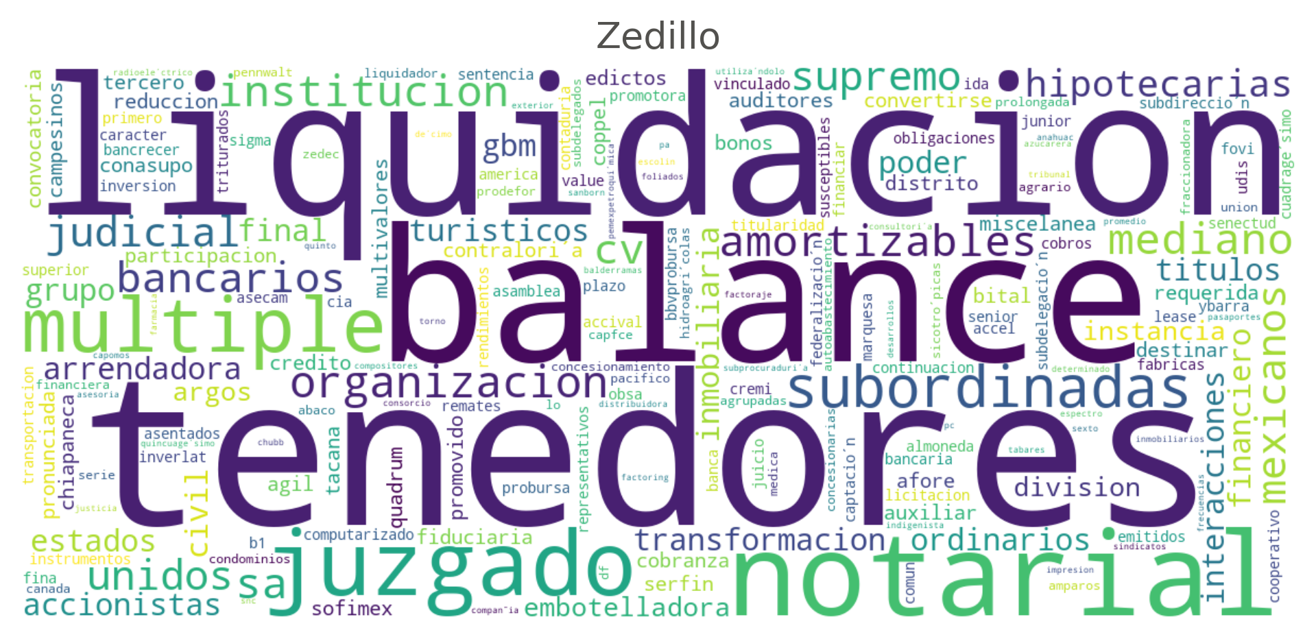
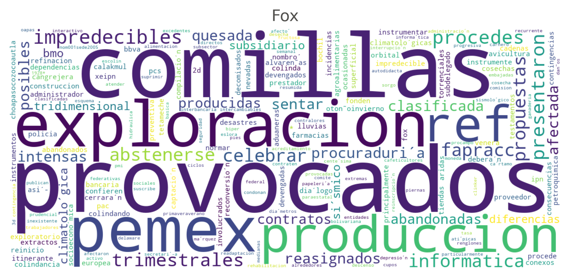
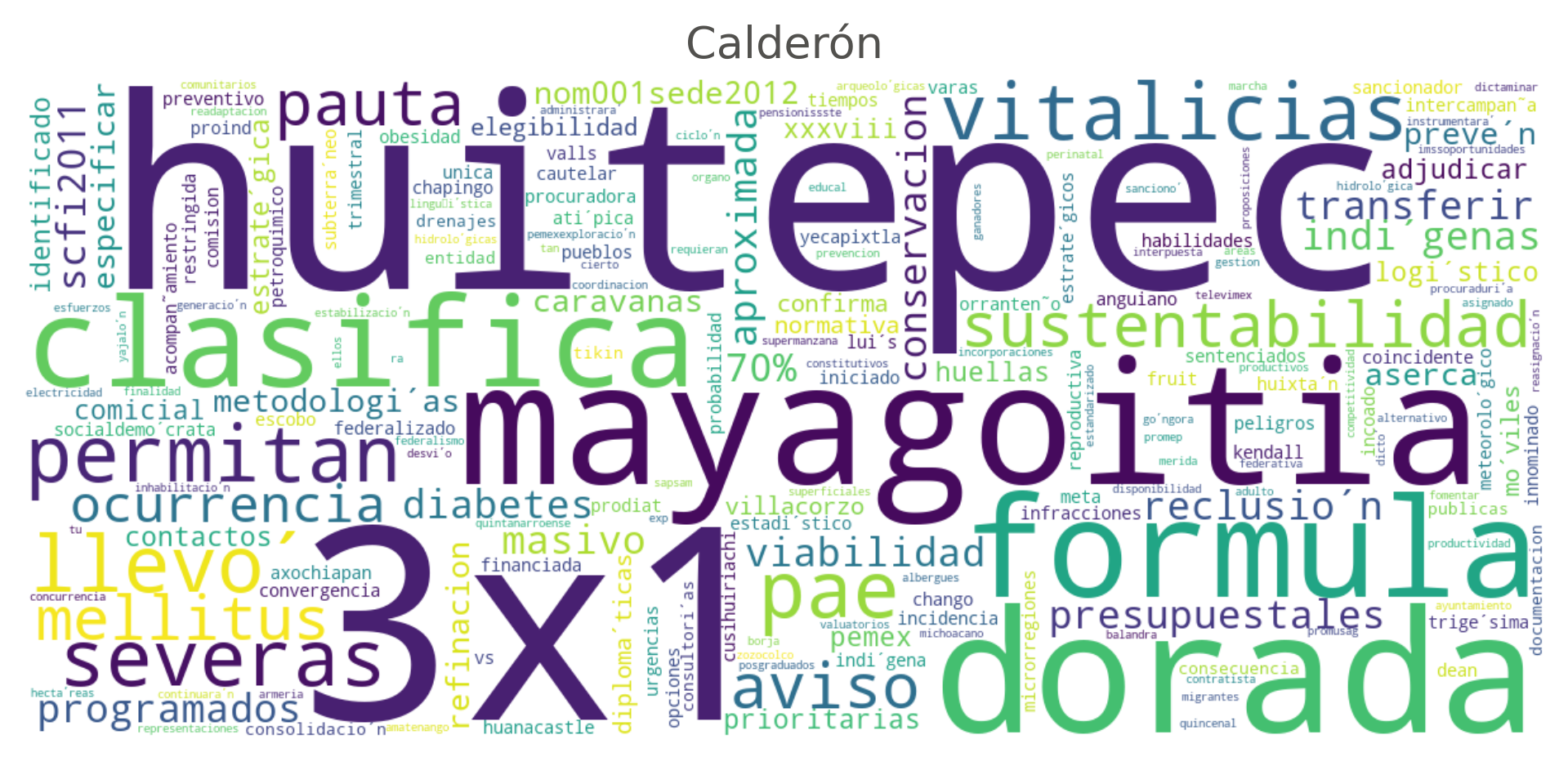
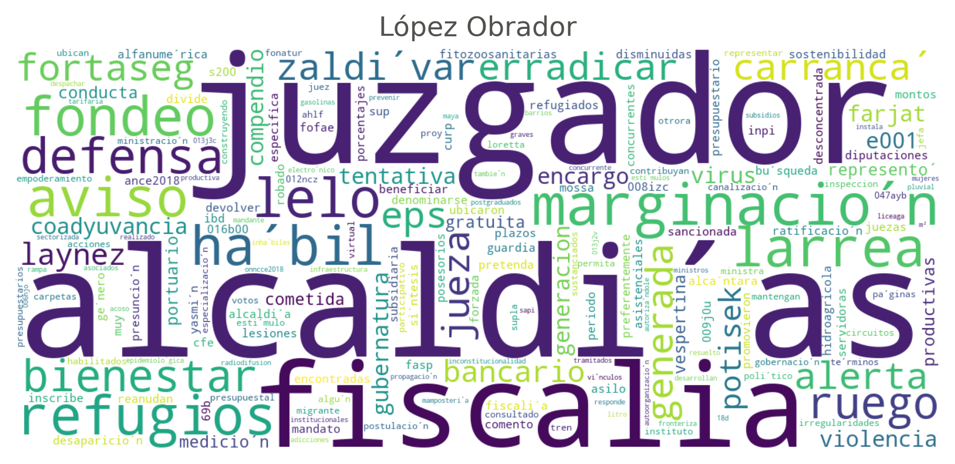
Mexican presidents have governed in fixed six-year terms — sexenios — since Lázaro Cárdenas (1934–1940). Grouping the titles by sexenio instead of by calendar year, and applying the very same pesos_discriminantes contrast, surfaces the vocabulary that sets an administration apart from the whole rest of the gazette. We look at four recent terms one at a time — Ernesto Zedillo, Vicente Fox, Felipe Calderón and Andrés Manuel López Obrador — each contrasted against every other title in the release: the other sexenios (including Peña Nieto’s and Sheinbaum’s, not shown) and everything before Zedillo, all folded into “the rest”, so no note is left out of the comparison. Since 2024 the start of the term moved from December 1 to October 1 (a 2014 constitutional reform), which is why López Obrador’s term ends two months short of six years.

Group the titles by presidential sexenio

import datetime as dt

SEXENIOS = [
    ("Zedillo",       dt.date(1994, 12, 1), dt.date(2000, 11, 30)),
    ("Fox",           dt.date(2000, 12, 1), dt.date(2006, 11, 30)),
    ("Calderón",      dt.date(2006, 12, 1), dt.date(2012, 11, 30)),
    ("Peña Nieto",    dt.date(2012, 12, 1), dt.date(2018, 11, 30)),
    ("López Obrador", dt.date(2018, 12, 1), dt.date(2024, 9, 30)),
    ("Sheinbaum",     dt.date(2024, 10, 1), dt.date(2030, 9, 30)),
]


def sexenio_de(fecha):
    """A note's sexenio, from its own `fecha`; anything earlier than Zedillo
    falls into "otros", so it still counts as part of "the rest" below."""
    d = dt.datetime.strptime(fecha, "%d-%m-%Y").date()
    for nombre, inicio, fin in SEXENIOS:
        if inicio <= d <= fin:
            return nombre
    return "otros"


# A second pass over the same cache: the titles are a stream, not a file, so
# a second grouping asks for the stream again rather than re-reading a dataset.
titles_by_sexenio = defaultdict(list)
for nota in legal_provisions_titles(log=lambda *_: None):
    titles_by_sexenio[sexenio_de(nota["fecha"])].append(nota["titulo"])

The same pesos_discriminantes function from above does the work: it neither knows nor cares whether its grouping is by year or by sexenio, only that titles_by_sexenio maps each sexenio’s name to its titles. A small helper draws one sexenio’s word cloud, and the four figures below call it in turn.

Helper: one sexenio’s word cloud

from wordcloud import WordCloud


def nube_sexenio(nombre):
    pesos = pesos_discriminantes(titles_by_sexenio, nombre, **params)
    wc = WordCloud(
        width=1200, height=520, background_color="white", random_state=42
    ).generate_from_frequencies(pesos)
    fig, ax = plt.subplots(figsize=(8, 4))
    ax.imshow(wc, interpolation="bilinear")
    ax.set_title(nombre, color=INK, fontsize=13)
    ax.axis("off")
    plt.show()

Code

nube_sexenio("Zedillo")

Figure 6: Terms that most identify Ernesto Zedillo’s sexenio (1994–2000) against the rest of the archive.

Code

nube_sexenio("Fox")

Figure 7: Terms that most identify Vicente Fox’s sexenio (2000–2006) against the rest of the archive.

Code

nube_sexenio("Calderón")

Figure 8: Terms that most identify Felipe Calderón’s sexenio (2006–2012) against the rest of the archive.

Code

nube_sexenio("López Obrador")

Figure 9: Terms that most identify Andrés Manuel López Obrador’s sexenio (2018–2024) against the rest of the archive.

8 What comes next

This exploration deliberately confined itself to the shallowest metadata in the archive, and even so the titles sufficed to date the digitization of the gazette, to measure the twilight of the land reform and to document the bureaucratization of its content. The tf-idf contrast behind those word clouds — by year and by presidential sexenio — is a first step toward the next installments: the automatic classification of the documentary types that the first word only approximates, and the full text of the notes, whose conversion to Markdown — with the nota2md and dof2md packages, now available on PyPI — is under way.

Methodological note

The data comes from the DOF’s open-data JSON service, queried day by day and republished as the notas-archivo GitHub release — one .tgz per year, plus one per month of the year still in progress — covering January 1, 1917 through June 30, 2026. A single call to dofjson.legal_provisions_titles streams every asset of that release (the daily index only, never the note contents) and feeds every figure and table on this page: the volume, first-word and length figures above — the last two segmented with the tokenize method of a microtc TextModel — Table 1 and Figure 4, both read off the codOrgaUno on every note plus the small codOrgaUno-to-name map the same pass fills in, and, further down, the word clouds, grouped by year and by presidential sexenio for the pesos_discriminantes tf-idf contrast (sexenio comparisons run against the whole release, with everything before Zedillo (1994) folded into “the rest”).

This exploration was carried out by the LegalIA team together with Claude, Anthropic’s coding assistant, through Claude Code: the assistant implemented the download-and-tf-idf pipeline behind the by-year and by-sexenio word clouds, produced the figures and drafted the accompanying analysis. The authors verified the resulting numbers against the archive and are responsible for the interpretations advanced here.