# Colab does not have CompStats preinstalled; it is installed only when it is missing.
# uv, which Colab provides, is much faster than pip; pip is the fallback.
try:
    import CompStats
except ImportError:
!uv pip install -q --system CompStats || pip install -q CompStatsCompetition Organizers
Ranking participants and reporting significance with CompStats

This page is aimed at people organizing a competition rather than at a single sklearn user. Given a gold standard and the predictions submitted by several participants, CompStats produces a ranking, confidence intervals for every submission, and p-values for the difference against the best submission. All of them come from the same paired bootstrap distribution, so the comparisons stay valid even when many participants are involved.
1 Dataset
The example uses the gold labels of INGEOTEC/Delitos, a corpus of tweets labeled as mentioning a crime (1) or not (0). Because the tweets’ text cannot be redistributed under Twitter/X’s terms of service, the published corpus only contains each tweet’s id and label. The following cell downloads the test partition and keeps the labels, which play the role of the gold standard an organizer would hold out from the competition’s participants.
import json
import urllib.request
import numpy as np

url = ("https://raw.githubusercontent.com/INGEOTEC/Delitos/main/"
       "corpus/delitos_test.json")
with urllib.request.urlopen(url) as fh:
    lines = fh.read().decode('utf-8').splitlines()
y_gold = np.array([json.loads(line)['label'] for line in lines])
y_gold.shape, y_gold.mean()
((360,), np.float64(0.2111111111111111))2 Simulated submissions
With only the labels available (no text to train a real classifier on), five submissions are simulated by flipping the gold label with a different probability per team. Higher skill means fewer flipped labels. Team Alpha and Team Beta share the same skill but flip different labels (a different random seed for each). Therefore, their predictions are not identical even though their expected performance is. They are meant to land in a statistical tie for first place. Team Gamma is a step below them but still competitive, and Team Delta and Team Epsilon trail further behind. This mirrors the kind of table an organizer receives, which has one column per participant, aligned with the same gold standard.
def simulate_submission(y_true, skill, seed):
    """A synthetic participant that mislabels with probability (1 - skill)"""
    rng = np.random.default_rng(seed)
    flip = rng.random(y_true.shape[0]) > skill
    y_pred = y_true.copy()
    y_pred[flip] = 1 - y_pred[flip]
    return y_pred

submissions = {
    'Team Alpha': simulate_submission(y_gold, skill=0.95, seed=0),
    'Team Beta': simulate_submission(y_gold, skill=0.95, seed=7),
    'Team Gamma': simulate_submission(y_gold, skill=0.90, seed=3),
    'Team Delta': simulate_submission(y_gold, skill=0.87, seed=2),
    'Team Epsilon': simulate_submission(y_gold, skill=0.86, seed=9),
}
3 Ranking the submissions
CompStats.metrics.f1_score follows the sklearn.metrics convention, that is, it takes (y_true, y_pred), and returns a Perf instance instead of a bare float. Passing every submission’s predictions, one call per team, builds the comparison and sorts it by performance. The bootstrap resampling draws its indices from NumPy’s global random state the first time it runs, so fixing the seed here makes the ranking, the confidence intervals, and the p-values below reproducible across runs of this notebook.
from CompStats.metrics import f1_score

np.random.seed(42)
leaderboard = None
for team, y_pred in submissions.items():
    if leaderboard is None:
        leaderboard = f1_score(y_gold, y_pred, name=team, pos_label=1)
    else:
        leaderboard(y_pred, name=team)
leaderboard
  0%|          | 0/5 [00:00<?, ?it/s]
 20%|██        | 1/5 [00:08<00:32,  8.18s/it]
 40%|████      | 2/5 [00:09<00:11,  3.91s/it]
 60%|██████    | 3/5 [00:10<00:05,  2.69s/it]
 80%|████████  | 4/5 [00:11<00:01,  1.89s/it]
100%|██████████| 5/5 [00:11<00:00,  1.46s/it]
100%|██████████| 5/5 [00:11<00:00,  2.34s/it]
<Perf(func=f1_score)>
Statistic with its standard error (se)
statistic (se)
0.9057 (0.0238) <= Team Beta
0.8554 (0.0296) <= Team Alpha
0.8263 (0.0318) <= Team Gamma
0.7500 (0.0350) <= Team Delta
0.7253 (0.0380) <= Team Epsilon4 Confidence intervals
Perf.ci reports the percentile bootstrap confidence interval for every submission’s F1 score, so the ranking above can be reported together with a measure of its uncertainty.
leaderboard.ci{'Team Delta': (np.float64(0.6771539721539722),
np.float64(0.8111514168658245)),
'Team Epsilon': (np.float64(0.6517443762781187),
np.float64(0.7978723404255319)),
'Team Gamma': (np.float64(0.7628125), np.float64(0.8780458698489652)),
'Team Alpha': (np.float64(0.7963957742272659),
np.float64(0.9086947456213511)),
'Team Beta': (np.float64(0.8540010141987829), np.float64(0.9493902439024389))}5 Significance against the best submission
Perf.difference compares every other submission against the best one (Team Beta here) using the paired bootstrap distribution of the differences, and Difference.p_value turns that distribution into a p-value per submission. Team Alpha’s p-value stays well above 0.05. Therefore, it is statistically tied with Team Beta for first place, even though the two teams’ predictions are not identical. Team Gamma, Team Delta, and Team Epsilon all trail the top two, but Team Gamma’s p-value sits close enough to the 0.05 boundary that, as the next section shows, the conclusion about it can change depending on how the p-values are corrected for testing four submissions against the best one at the same time.
comparison = leaderboard.difference()
comparison
<Difference>
difference p-values w.r.t Team Beta
0.0000 <= Team Delta
0.0000 <= Team Epsilon
0.0180 <= Team Gamma
0.0880 <= Team Alphacomparison.p_value(){'Team Delta': np.float64(0.0),
'Team Epsilon': np.float64(0.0),
'Team Gamma': np.float64(0.018),
'Team Alpha': np.float64(0.088)}6 Correcting for multiple comparisons
Every submission other than the best is tested in the same round, so judging four hypotheses at once against an uncorrected 0.05 threshold inflates the chance that at least one “significant” difference is actually a false positive, which is the familywise error rate. Difference.p_value’s correction argument adjusts for this using any method supported by statsmodels.stats.multitest.multipletests. Three common choices are 'bonferroni' (multiplies every p-value by the number of comparisons, which is simple and the most conservative of the three), 'holm' (a step-down version of Bonferroni that is less conservative), and 'fdr_bh' (Benjamini-Hochberg, which bounds the expected proportion of false positives among the rejected hypotheses rather than the probability of any single false positive, making it the least conservative of the three).
import pandas as pd

pd.DataFrame({
    'raw': comparison.p_value(),
    'bonferroni': comparison.p_value(correction='bonferroni'),
    'holm': comparison.p_value(correction='holm'),
    'fdr_bh': comparison.p_value(correction='fdr_bh'),
})| raw | bonferroni | holm | fdr_bh | |
|---|---|---|---|---|
| Team Delta | 0.000 | 0.000 | 0.000 | 0.000 |
| Team Epsilon | 0.000 | 0.000 | 0.000 | 0.000 |
| Team Gamma | 0.018 | 0.072 | 0.036 | 0.024 |
| Team Alpha | 0.088 | 0.352 | 0.088 | 0.088 |
Team Gamma’s p-value crosses the 0.05 threshold depending on the method. Under the raw p-value, Holm, and the FDR correction it stays significantly behind the top two, but Bonferroni’s stricter correction is enough to call it statistically tied with them instead. The clear-cut cases are unaffected by the choice. Team Alpha remains tied with Team Beta and Team Delta and Team Epsilon remain clearly behind under every correction.
7 Visualizing the comparison
Perf.plot and Difference.plot color every submission by whether it is the best, tied with the best, or significantly behind it, with confidence intervals computed from the same bootstrap distribution. Passing the same correction argument used above recomputes that coloring from the corrected p-values.
leaderboard.plot()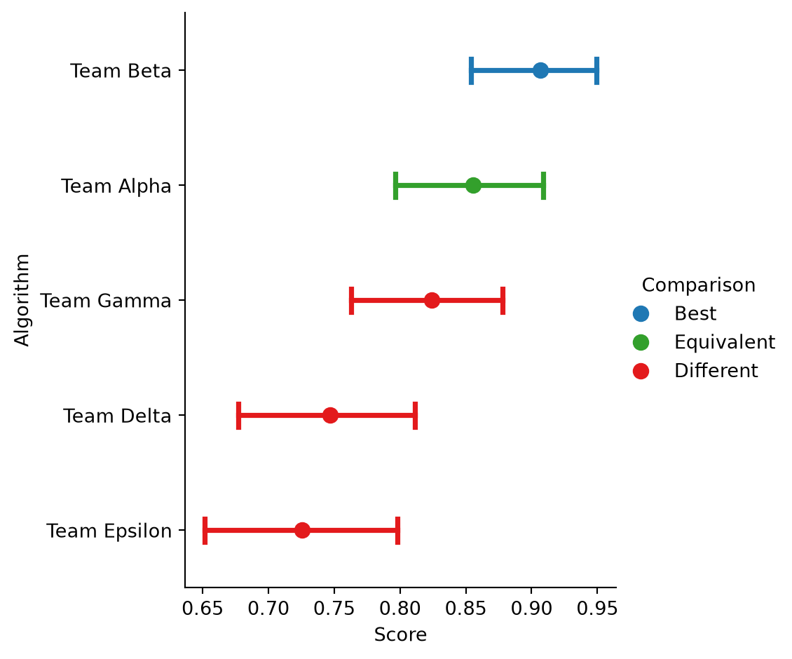
comparison.plot()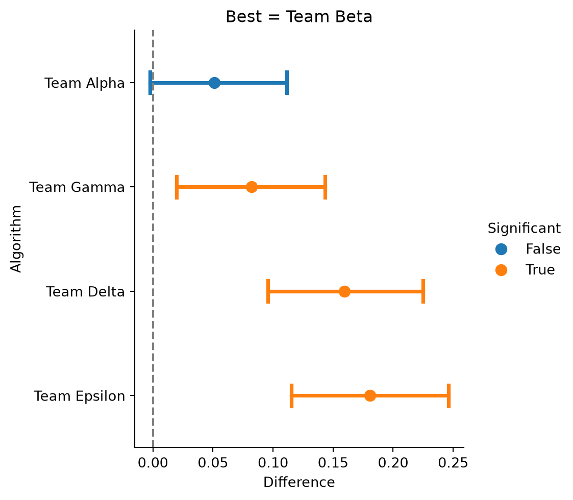
Requesting correction='bonferroni' recolors Team Gamma from “behind” to “tied” in both plots below, since Bonferroni is the only one of the three corrections that pushes its p-value past 0.05. 'holm' and 'fdr_bh' can be passed the same way, but neither changes any submission’s color in this comparison. Their corrected p-values for Team Gamma stay under 0.05, so the plots would look identical to the uncorrected ones above.
leaderboard.plot(correction='bonferroni')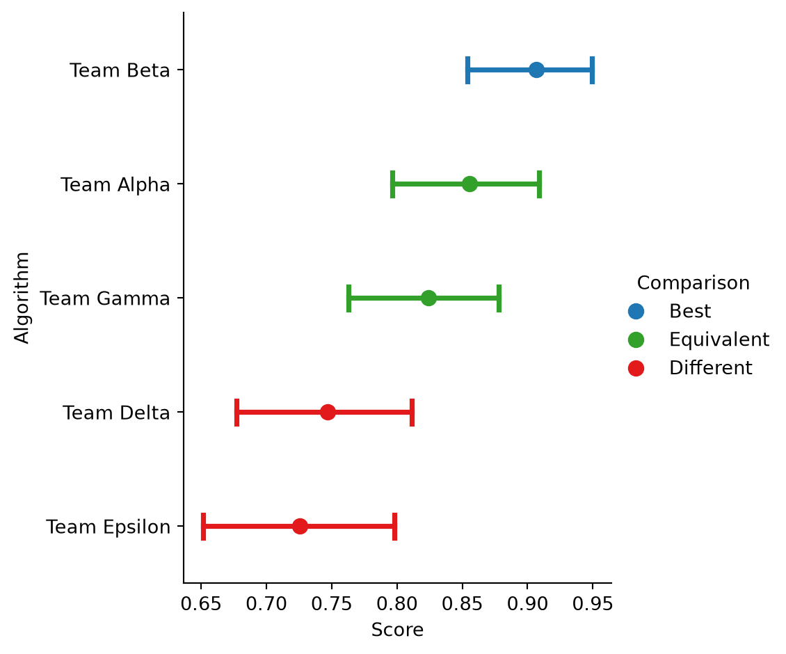
comparison.plot(correction='bonferroni')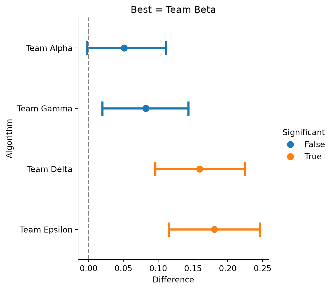
scikit-learn Users shows the same workflow when comparing a handful of estimators against a single gold standard, and Multiple Testing shows how to combine several measures in a single Perf and correct their p-values.