# Colab does not have CompStats preinstalled; it is installed only when it is missing.
# uv, which Colab provides, is much faster than pip; pip is the fallback.
try:
    import CompStats
except ImportError:
!uv pip install -q --system CompStats || pip install -q CompStatsscikit-learn Users
A quick guide to comparing the predictions of scikit-learn models with CompStats

To illustrate the use of CompStats, the following example loads a classification problem (the digits dataset), trains four different classifiers, and uses CompStats.metrics.f1_score to measure and compare their performance. As with the rest of sklearn.metrics, the score function takes (y_true, y_pred). The difference is that it returns a Perf instance, with the standard error, confidence interval, and pairwise significance tests already computed from the bootstrap distribution. The package is not limited to classification. The last section, Regression, repeats the comparison with three regressors and an error measure.
1 Dataset and libraries
The first step is to load the digits dataset and split it into a training (X_train, y_train) and a validation set (X_val, y_val).
import numpy as np
from sklearn.svm import LinearSVC
from sklearn.naive_bayes import GaussianNB
from sklearn.ensemble import RandomForestClassifier
from sklearn.ensemble import HistGradientBoostingClassifier
from sklearn.datasets import load_digits
from sklearn.model_selection import train_test_split
from CompStats.metrics import f1_score

X, y = load_digits(return_X_y=True)
_ = train_test_split(X, y, test_size=0.3, random_state=0)
X_train, X_val, y_train, y_val = _
2 Linear SVM
The following line trains a linear Support Vector Machine and predicts the validation set’s classes. The predictions are stored in hy.
m = LinearSVC(random_state=0).fit(X_train, y_train)
hy = m.predict(X_val)
3 Score
Once the predictions are available, f1_score measures the classifier’s performance. The API follows the sklearn.metrics convention, that is, the function takes (y_true, y_pred), but the result, score, is a Perf instance rather than a bare float.
np.random.seed(0)
score = f1_score(y_val, hy, name='Linear SVM', average='macro')
score
  0%|          | 0/1 [00:00<?, ?it/s]
100%|██████████| 1/1 [00:09<00:00,  9.07s/it]
100%|██████████| 1/1 [00:09<00:00,  9.08s/it]
<Perf(func=f1_score, statistic=0.9440, se=0.0098)>The printed representation of score shows two values. statistic is the measure computed on the validation set, here the macro-\(F_1\) of the linear SVM. It is the number that sklearn.metrics.f1_score returns for the same arguments, and it is available as score.statistic. se is the standard error of that measure, estimated as the standard deviation of the measure over the bootstrap samples of the validation set (500 by default, parameter num_samples). It is available as score.se. The standard error quantifies how much the measure would vary if the validation set were another sample of the same population. The confidence interval, by default at the 95% level, is in score.ci.
4 Random Forest
Comparing a second classifier against the same gold standard reuses the same bootstrap resamples. Calling score with a new set of predictions adds them to the comparison without redrawing the bootstrap, keeping every pairwise comparison paired.
ens = RandomForestClassifier(random_state=0).fit(X_train, y_train)
score(ens.predict(X_val), name='Random Forest')
  0%|          | 0/1 [00:00<?, ?it/s]
100%|██████████| 1/1 [00:00<00:00,  1.79it/s]
100%|██████████| 1/1 [00:00<00:00,  1.79it/s]
<Perf(func=f1_score)>
Statistic with its standard error (se)
statistic (se)
0.9783 (0.0061) <= Random Forest
0.9440 (0.0098) <= Linear SVM5 Rest of the classifiers
Adding a Naive Bayes classifier and a Histogram Gradient Boosting Tree completes the comparison. Perf.plot renders all four systems’ performance together with their confidence intervals.
nb = GaussianNB().fit(X_train, y_train)
_ = score(nb.predict(X_val), name='Naive Bayes')
hist = HistGradientBoostingClassifier(random_state=0).fit(X_train, y_train)
_ = score(hist.predict(X_val), name='Hist. Grad. Boost. Tree')
score.plot()
  0%|          | 0/2 [00:00<?, ?it/s]
 50%|█████     | 1/2 [00:00<00:00,  1.60it/s]
100%|██████████| 2/2 [00:01<00:00,  1.25it/s]
100%|██████████| 2/2 [00:01<00:00,  1.29it/s]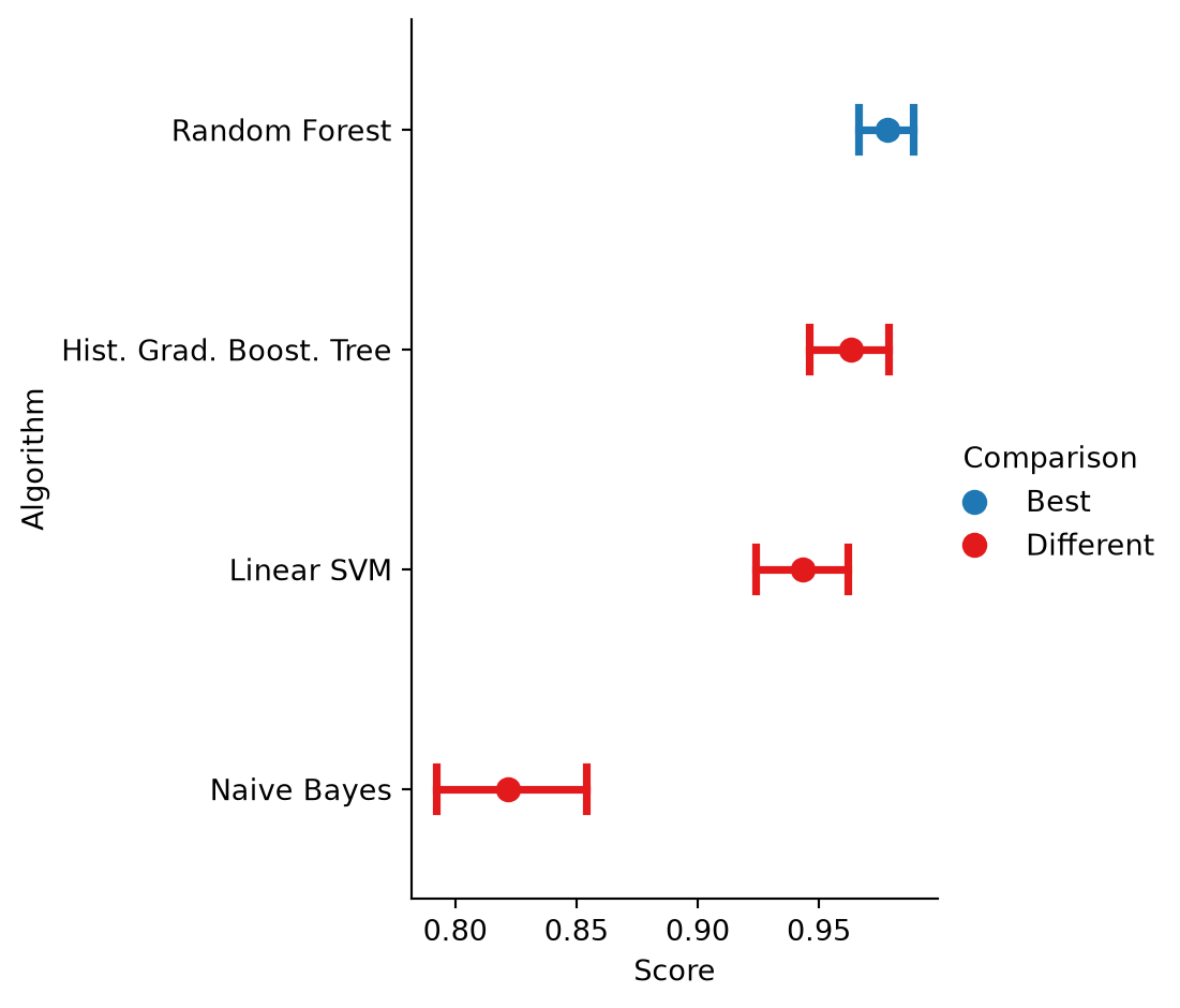
In the figure, each row is a classifier, and the classifiers are ordered from the best, at the top, to the worst. The dot is the mean of the bootstrap distribution of the measure, and the horizontal bar is its 95% confidence interval. The colour is the result of comparing each classifier with the best one, which is drawn in blue, with the paired bootstrap test described in Methodology. A classifier is Equivalent (green) when its difference with the best one is not statistically significant at the 0.05 level, and Different (red) when it is. In this example the random forest is the best classifier and the other three are statistically different from it. The p-values behind the colours are obtained in the next section.
The data split, the classifiers and NumPy’s global random state, from which the bootstrap samples are drawn, are seeded so that this page is reproducible.
6 Comparison against the best system
Perf.difference computes, on the same bootstrap samples, the difference between the best system and each of the others. The object it returns prints the p-value of each difference.
diff = score.difference()
diff
<Difference>
difference p-values w.r.t Random Forest
0.0000 <= Linear SVM
0.0000 <= Naive Bayes
0.0060 <= Hist. Grad. Boost. Tree7 Correction for multiple comparisons
Three systems are compared with the best one at the same time, so the p-values are adjusted for multiple comparisons, here with Holm’s method. The correction is described in more detail in Multiple Testing.
diff.p_value(correction='holm'){'Linear SVM': np.float64(0.0),
'Naive Bayes': np.float64(0.0),
'Hist. Grad. Boost. Tree': np.float64(0.006)}Difference.plot draws the confidence interval of each difference. An interval that contains zero means that the system is not statistically different from the best one.
diff.plot()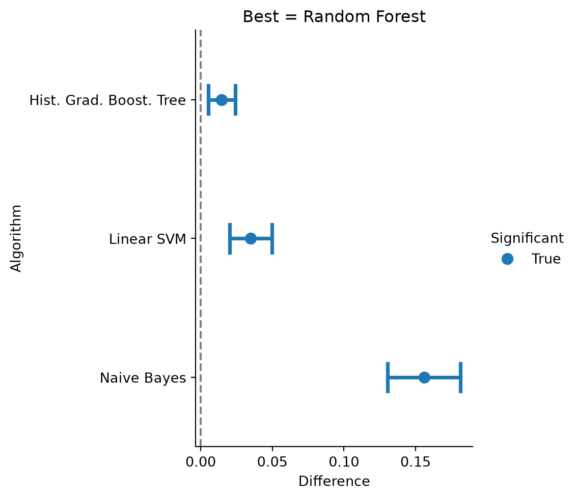
8 Regression
The same workflow applies to regression problems. The following example loads the diabetes dataset, trains three regressors and compares them with CompStats.metrics.mean_absolute_error. For this measure a smaller value is better. Every function of CompStats.metrics knows the direction of its measure, so the best system is the one with the smallest error and nothing else changes in the code.
from sklearn.datasets import load_diabetes
from sklearn.linear_model import LinearRegression
from sklearn.ensemble import RandomForestRegressor
from sklearn.ensemble import HistGradientBoostingRegressor
from CompStats.metrics import mean_absolute_error

X, y = load_diabetes(return_X_y=True)
_ = train_test_split(X, y, test_size=0.3, random_state=0)
X_train, X_val, y_train, y_val = _

np.random.seed(0)
lr = LinearRegression().fit(X_train, y_train)
error = mean_absolute_error(y_val, lr.predict(X_val), name='Linear Regression')
forest = RandomForestRegressor(random_state=0).fit(X_train, y_train)
_ = error(forest.predict(X_val), name='Random Forest')
hist = HistGradientBoostingRegressor(random_state=0).fit(X_train, y_train)
_ = error(hist.predict(X_val), name='Hist. Grad. Boost. Tree')
error
  0%|          | 0/3 [00:00<?, ?it/s]
 33%|███▎      | 1/3 [00:00<00:01,  1.35it/s]
 67%|██████▋   | 2/3 [00:01<00:00,  1.22it/s]
100%|██████████| 3/3 [00:02<00:00,  1.20it/s]
100%|██████████| 3/3 [00:02<00:00,  1.21it/s]
<Perf(func=mean_absolute_error)>
Statistic with its standard error (se)
statistic (se)
44.6176 (2.8668) <= Linear Regression
46.5703 (3.3280) <= Hist. Grad. Boost. Tree
47.7996 (2.9929) <= Random ForestThe systems are listed from the smallest to the largest error. Perf.plot and Perf.difference are used exactly as in the classification example. The horizontal axis of the figure is now labelled as an error, and the best system, at the top, is the one with the smallest error.
error.plot()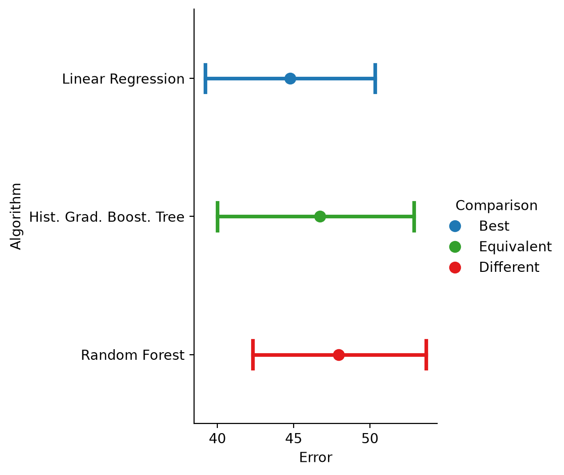
In the figure, the histogram gradient boosting tree is statistically equivalent to the linear regression, whereas the random forest is marked as different. The colours of Perf.plot come from p-values that are not corrected for multiple comparisons unless its correction argument is given. The p-values of the differences with respect to the best regressor, adjusted with Holm’s method, are obtained as before. With the correction, neither difference is significant at the 0.05 level.
error.difference().p_value(correction='holm'){'Random Forest': np.float64(0.052),
'Hist. Grad. Boost. Tree': np.float64(0.166)}Competition Organizers extends this workflow to ranking many participants against a gold standard, and Multiple Testing shows how to combine several measures in a single Perf and correct their p-values.