# Colab does not have CompStats preinstalled; it is installed only when it is missing.
# uv, which Colab provides, is much faster than pip; pip is the fallback.
try:
    import CompStats
except ImportError:
!uv pip install -q --system CompStats || pip install -q CompStatsMultiple Testing
A quick guide to comparing several performance measures and correcting their p-values

This page is aimed at anyone who needs to compare systems on more than one performance measure at once, e.g., precision together with recall, rather than settling for a single score. CompStats.interface.Perf can hold several measures in one instance, evaluated on the same paired bootstrap distribution, so the comparisons stay consistent across measures. Difference.p_value’s correction argument then adjusts for testing several hypotheses at the same time, whether those hypotheses come from several systems, several measures, or both.
1 Dataset
Three synthetic submissions are built from the same gold standard, each with a different precision/recall trade-off: precise predicts the positive class conservatively (few false positives, more missed positives), broad predicts it liberally (catches almost every positive, but with more false alarms), and balanced sits between the two. The trade-off is controlled directly by each system’s false-positive and false-negative rates, so the example does not depend on training an actual classifier.
import numpy as np

def make_system(y_true, fp_rate, fn_rate, seed):
    """A synthetic system that mislabels negatives/positives at the given rates"""
    rng = np.random.default_rng(seed)
    y_pred = y_true.copy()
    pos_idx = np.where(y_true == 1)[0]
    neg_idx = np.where(y_true == 0)[0]
    y_pred[pos_idx[rng.random(pos_idx.shape[0]) < fn_rate]] = 0
    y_pred[neg_idx[rng.random(neg_idx.shape[0]) < fp_rate]] = 1
    return y_pred

rng = np.random.default_rng(0)
y_gold = (rng.random(400) < 0.5).astype(int)
precise = make_system(y_gold, fp_rate=0.02, fn_rate=0.30, seed=1)
broad = make_system(y_gold, fp_rate=0.30, fn_rate=0.02, seed=2)
balanced = make_system(y_gold, fp_rate=0.11, fn_rate=0.13, seed=3)
2 Comparing three performance measures at once
Passing a list of functions to Perf’s func argument combines them into a single, multi-measure instance, here precision_score, recall_score, and f1_score from CompStats.metrics. Each of them is built with its .measure factory so that its BiB tag (bigger is better, for all three) travels with it. measure_names labels the columns of the result. As with a single-measure Perf, fixing the seed makes the bootstrap resampling below reproducible.
from CompStats.metrics import precision_score, recall_score, f1_score
from CompStats.interface import Perf

np.random.seed(42)
perf = Perf(y_gold, precise=precise, broad=broad, balanced=balanced,
            func=[precision_score.measure(pos_label=1),
                  recall_score.measure(pos_label=1),
                  f1_score.measure(pos_label=1)],
            measure_names=['Precision', 'Recall', 'F1'])
perf
  0%|          | 0/3 [00:00<?, ?it/s]
 33%|███▎      | 1/3 [00:11<00:23, 11.60s/it]
 67%|██████▋   | 2/3 [00:12<00:05,  5.48s/it]
100%|██████████| 3/3 [00:13<00:00,  3.50s/it]
100%|██████████| 3/3 [00:13<00:00,  4.65s/it]
<Perf(func=Precision+Recall+F1)>
Statistic with its standard error (se)
statistic (se)
0.8859 (0.0245), 0.8907 (0.0239), 0.8883 (0.0190) <= balanced
0.9776 (0.0129), 0.7158 (0.0332), 0.8265 (0.0229) <= precise
0.7149 (0.0306), 0.9727 (0.0120), 0.8241 (0.0211) <= broad3 Best system per measure
Perf.best reports the top system for every measure, and the three systems split the wins exactly as their construction intends: precise leads on Precision, broad leads on Recall, and balanced, which is not the best at either individual measure, comes out ahead once Precision and Recall are combined into F1. Note that best only compares point estimates. It says nothing about whether the lead is statistically significant, which is exactly what the next section checks.
perf.bestarray(['precise', 'broad', 'balanced'], dtype='<U8')4 p-values per measure
Perf.difference() still produces a Difference instance from the same paired bootstrap distribution, and Difference.p_value() now returns one array per system, with one entry per measure.
import pandas as pd

diff = perf.difference()
pd.DataFrame(diff.p_value(), index=perf.measure_names).T| Precision | Recall | F1 | |
|---|---|---|---|
| balanced | 0.0 | 0.004 | 1.000 |
| broad | 0.0 | 1.000 | 0.008 |
| precise | 1.0 | 0.000 | 0.022 |
precise and broad are each other’s clear runner-up on the measure the other wins (Recall and Precision, respectively), with a p-value of essentially 0. The interesting row is F1. Both precise and broad trail balanced with uncorrected p-values under 0.05 (0.022 and 0.008), so a naive reading would call balanced significantly ahead of both. But three measures were just tested against balanced at once, so before trusting that F1 conclusion, the next section checks whether it survives a correction for multiple comparisons.
5 Correcting for multiple comparisons
Difference.p_value’s correction argument passes any method supported by statsmodels.stats.multitest.multipletests (e.g., 'bonferroni', 'holm', 'fdr_bh') and, with several measures, corrects each measure independently (i.e., per column), so one metric’s correction never mixes with another’s. The following table focuses on the F1 column, comparing the raw p-values against the three correction methods.
pd.DataFrame({
    'raw': {k: v[2] for k, v in diff.p_value().items()},
    'bonferroni': {k: v[2] for k, v in diff.p_value(correction='bonferroni').items()},
    'holm': {k: v[2] for k, v in diff.p_value(correction='holm').items()},
    'fdr_bh': {k: v[2] for k, v in diff.p_value(correction='fdr_bh').items()},
})| raw | bonferroni | holm | fdr_bh | |
|---|---|---|---|---|
| balanced | 1.000 | 1.000 | 1.000 | 1.000 |
| broad | 0.008 | 0.024 | 0.024 | 0.024 |
| precise | 0.022 | 0.066 | 0.044 | 0.033 |
broad stays significantly behind balanced on F1 under every method. precise, however, crosses the 0.05 threshold depending on the correction. Bonferroni’s stricter adjustment (0.066) is enough to call it statistically tied with balanced on F1, while Holm (0.044) and the FDR correction (0.033) both keep it significantly behind. This is the same lesson as Competition Organizers’s Team Gamma, except the extra hypothesis being tested here comes from combining measures rather than from ranking more systems.
6 Visualizing the comparison
Perf.plot renders one panel per measure, coloring each system by whether it is the best, tied with the best, or significantly behind it on that measure. Therefore, the three-way split from perf.best above is visible directly, alongside each system’s confidence interval.
perf.plot()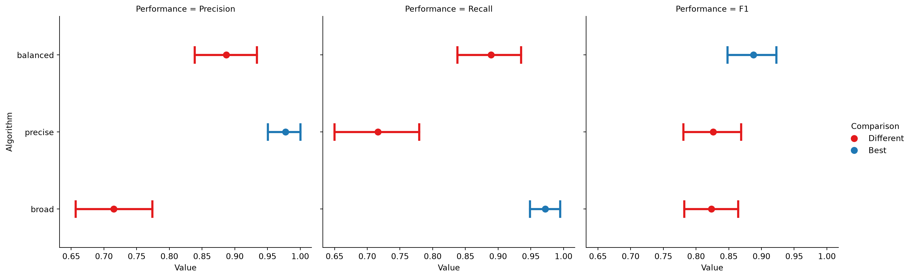
Difference.plot shows the same paired differences against each measure’s best system, coloring by statistical significance instead.
diff.plot()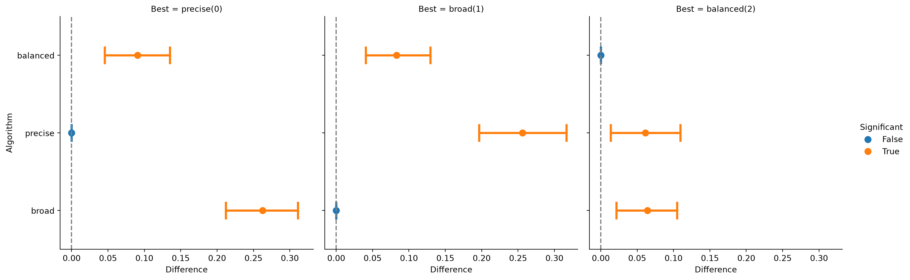
Passing correction='bonferroni' recolors precise’s F1 panel from significantly behind to tied in both plots, matching the table above. 'holm' and 'fdr_bh' would leave every panel unchanged from the uncorrected plots, since neither pushes precise’s F1 p-value past 0.05.
perf.plot(correction='bonferroni')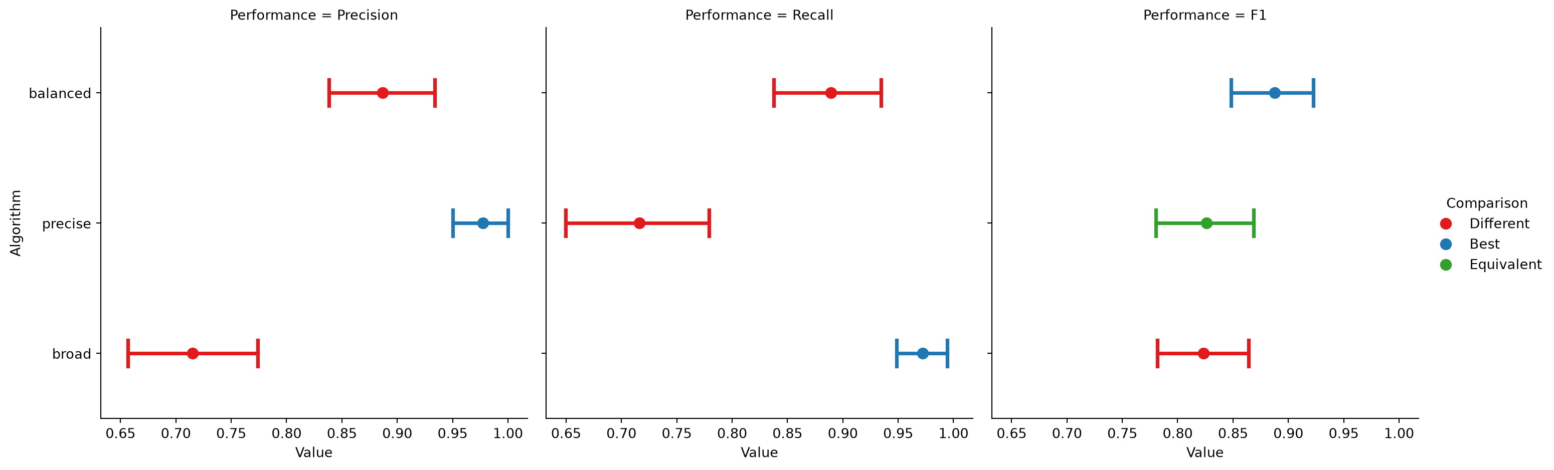
diff.plot(correction='bonferroni')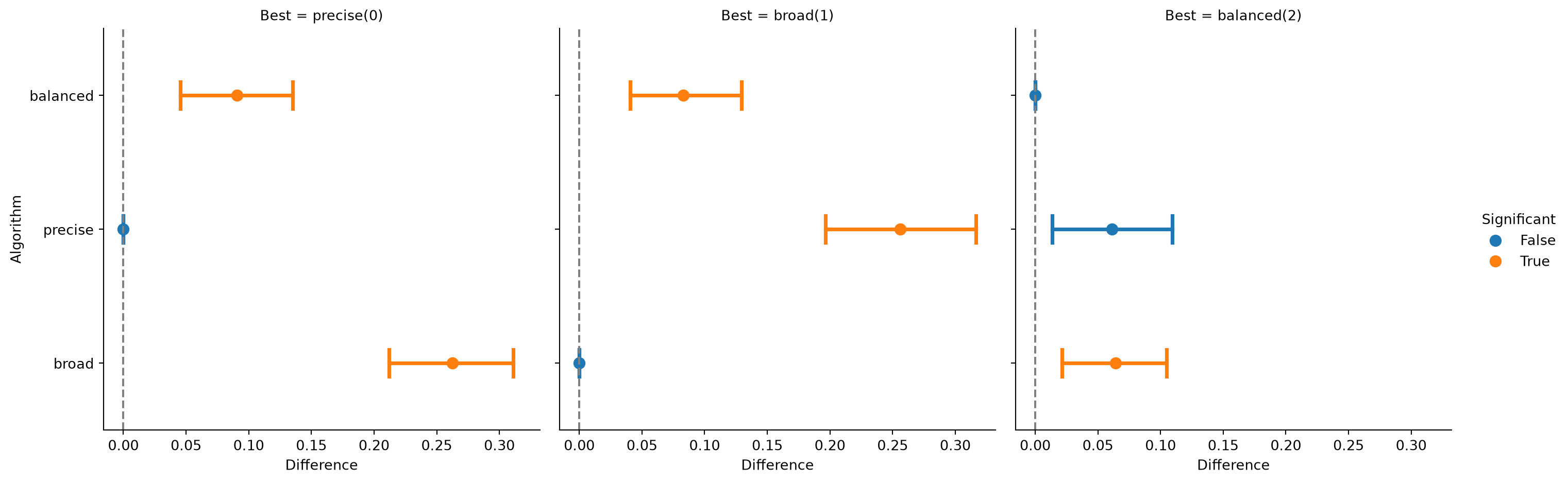
scikit-learn Users and Competition Organizers show this same workflow with a single performance measure, comparing a handful of estimators or ranking many competition submissions against a shared gold standard.