Vocabulary Laws
Contents
Libraries used
from microtc.utils import tweet_iterator
from EvoMSA.tests.test_base import TWEETS
from text_models import Vocabulary
from text_models.utils import date_range
from wordcloud import WordCloud as WC
import numpy as np
from collections import Counter
from matplotlib import pylab as plt
from scipy.optimize import minimize
from joblib import Parallel, delayed
from tqdm import tqdm
Installing external libraries
pip install microtc
pip install evomsa
pip install text_models
Introduction
The journey of natural language processing starts with the simple procedure of counting words; with it, we will be able to model some characteristics of the languages, identify patterns in a text, and perform exploratory data analysis on a collection of Tweets.
At this point, let us define a word as a sequence of characters bounded by a space - this is a shallow definition; however, it is suitable for most words written in Latin languages and English.
Frequency of the words
The frequency of the words in a document can be computed using a dictionary. A dictionary is a data structure that associates a keyword with a value. The following code uses a dictionary (variable word) to count the word frequencies of texts stored in a JSON format, each one per line. It uses the function tweet_iterator that iterates over the file, scanning one line at a time and converting the JSON into a dictionary where the keyword text contains the text.
words = dict()
for tw in tweet_iterator(TWEETS):
    text = tw['text']
    for w in text.split():
        key = w.strip()
        try:
            words[key] += 1
        except KeyError:
            words[key] = 1
Method split returns a list of strings where the split occurs on the space character, which follows the definition of a word. Please note the use of an exception to handle the case where the keyword is not in the dictionary. As an example, the word si (yes in Spanish) appears 29 times in the corpus.
words['si']
29
The counting pattern is frequent, so it is implemented in the Counter class under the package collections; the following code implements the method described using Counter; the key element is the method update, and to make the code shorter, list comprehension is used.
words = Counter()
for tw in tweet_iterator(TWEETS):
    text = tw['text']
    words.update([x.strip() for x in text.split()])
Counter has another helpful method to analyze the frequencies; in particular, the most_common method returns the most frequent keywords. For example, the following code gets the five most common keywords.
words.most_common(5)
[('de', 299), ('que', 282), ('a', 205), ('la', 182), ('el', 147)]
These are the words, of, what, a, the, and the, respectively.
Zipf’s Law
The word frequency allows defining some empirical characteristics of the language. These characteristics are essential to understand the challenges of developing an algorithm capable of understanding language.
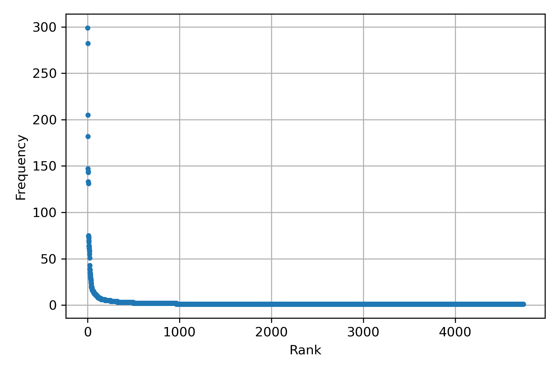
Let us start with Zipf’s law. The law relates the frequency of a word with its rank. In an order set, the rank corresponds to the element’s position, e.g., the first element has the rank of one, the second has the second rank, and so on. Explicitly, the relationship is defined as \(f \cdot r = c\), where \(f\) is the frequency, \(r\) is the rank, and \(c\) is a constant. For example, the frequency is \(f=\frac{c}{r}\); as can be seen when the rank equals the constant, then the frequency is one, meaning that the rest of the words are infrequent and that there are only frequent few words.
The following figure depicts the described characteristic. It shows a scatter plot between rank and frequency.
The frequency and the rank can be computed with the following two lines using the dataset of the previous example.
freq = [f for _, f  in words.most_common()]
rank = range(1, len(freq) + 1)
Once the frequency and the rank are computed, the figure is created using the following code.
plt.plot(rank, freq, '.')
plt.grid()
plt.xlabel('Rank')
plt.ylabel('Frequency')
plt.tight_layout()
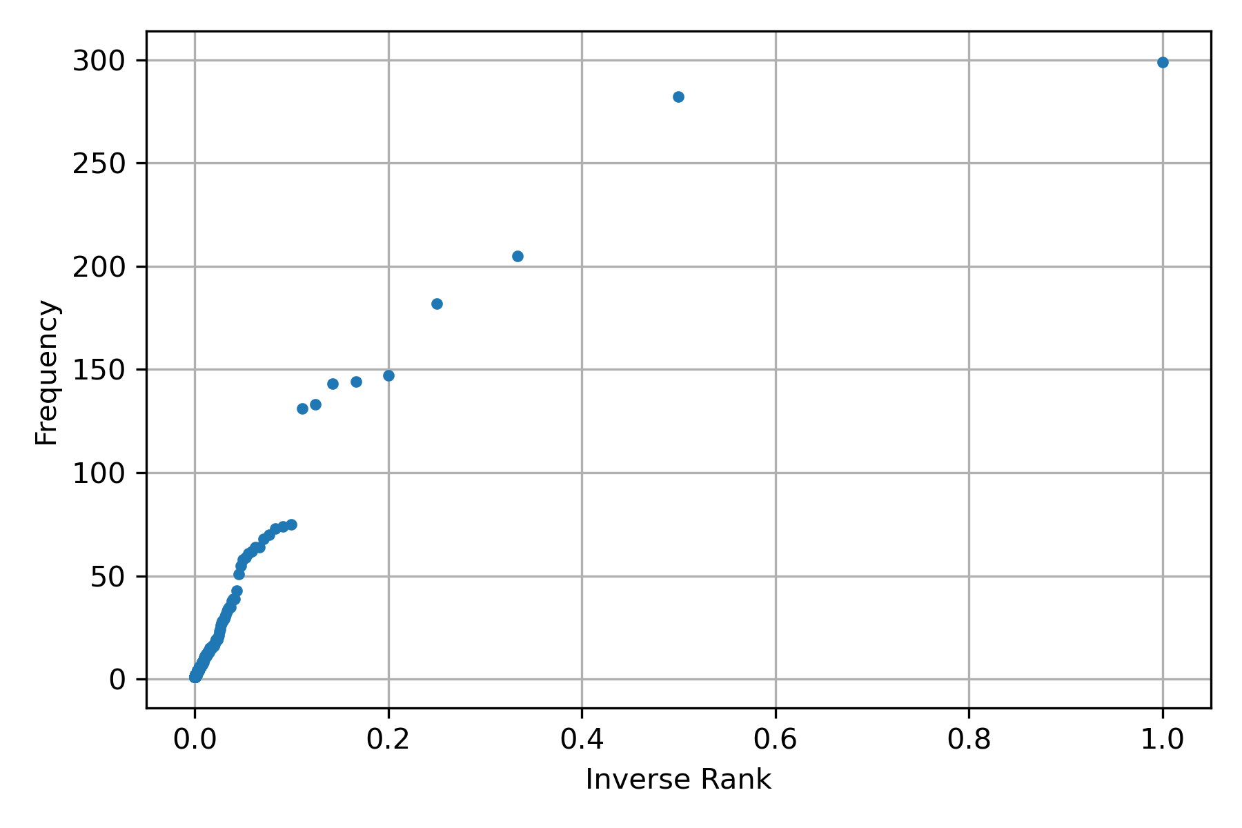
The previous figure does not depict the relation \(f=\frac{c}{r}\), in order to show it let us draw the figure scatter plot between the rank inverse and the frequency; this can be obtained by changing the following lines into the previous procedure – numpy is used in the following code to create an array of elements.
freq = [f for _, f  in words.most_common()]
rank = 1 / np.arange(1, len(freq) + 1)
As observed from the following figure, Zipf’s Law is a rough estimate of the relationship between rank and frequency. Nonetheless, it provides all the elements to understand the importance of this relationship.
Ordinary Least Squares
The missing step is to estimate the value of \(c\). Constant \(c\) can be calculated using ordinary least squares (OLS). The idea is to create a system of equations where the unknown is \(c\), and the dependent variable is \(f\). These can represent in matrix notation as \(A \cdot \mathbf c = \mathbf f\), where \(A \in \mathbb R^{N \times 1}\) is composed by \(N\) inverse rank measurements, \(c \in \mathbb R^1\) is the parameter to be identified, and \(\mathbf f \in \mathbb R^N\) is a column vector containing the frequency measurements.
The coefficients can be computed using the function np.linalg.lstsq described in the following code.
X = np.atleast_2d(rank).T
c = np.linalg.lstsq(X, freq, rcond=None)[0]
c
array([461.40751913])
Once \(c\) has been identified, it can be used to predict the model; the following figure presents the measurements and the predicted points using the identified coefficient.
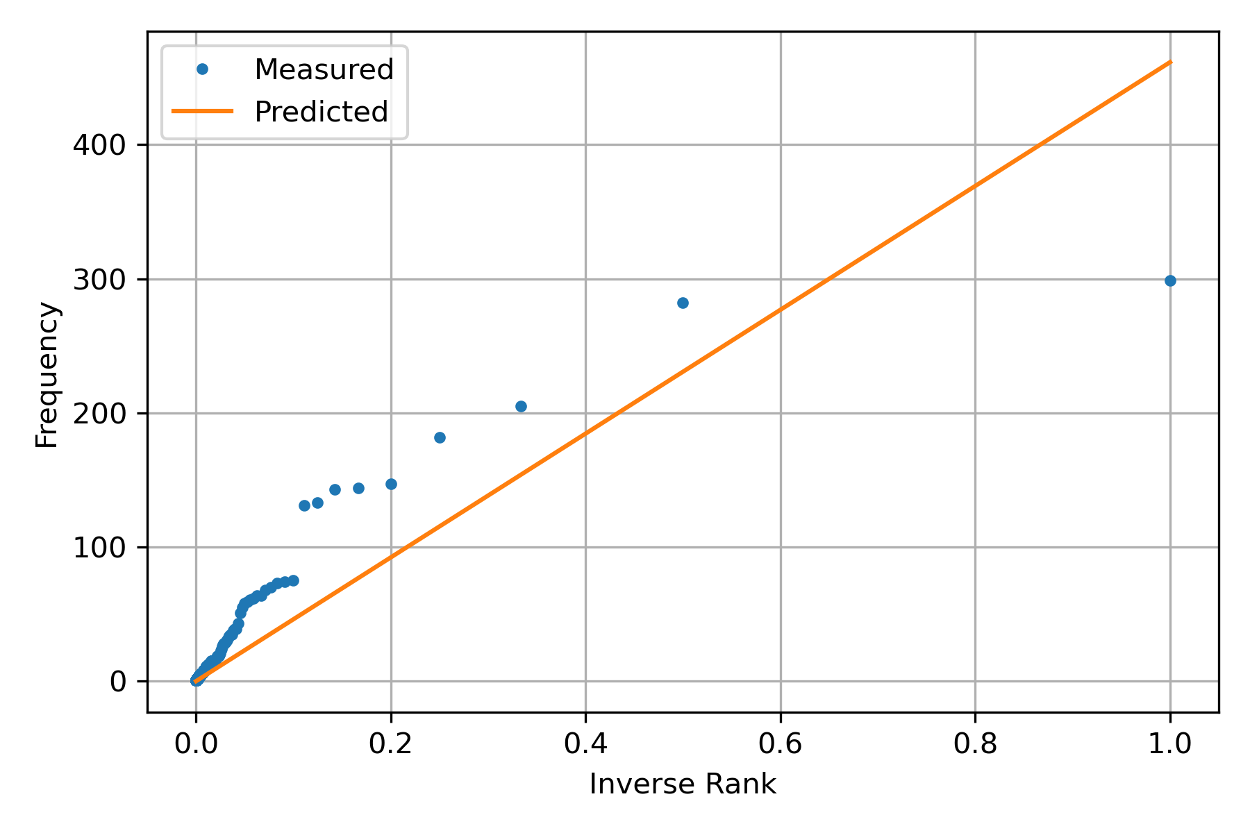
The previous figure was created with the following code; the variable hy contains the predicted frequency.
hy = np.dot(X, c)
plt.plot(rank, freq, '.')
plt.plot(rank, hy)
plt.legend(['Measured', 'Predicted'])
plt.grid()
plt.xlabel('Inverse Rank')
plt.ylabel('Frequency')
plt.tight_layout()
Herdan’s Law / Heaps’ Law
A language used evolves new words are incorporated in the language, and the relationship between the vocabulary size and the number of words (tokens) is expressed in the Heaps’ Law. Let \(\mid v \mid\) represents the vocabulary size, and \(n\) the number of words; then the relationship between these elements is \(\mid v \mid = k n^\beta\) where \(k\) and \(\beta\) are the parameters that need to be identified.
The following figure depicts the relation between \(n\) and \(\mid v \mid\) using the dataset of the previous examples.
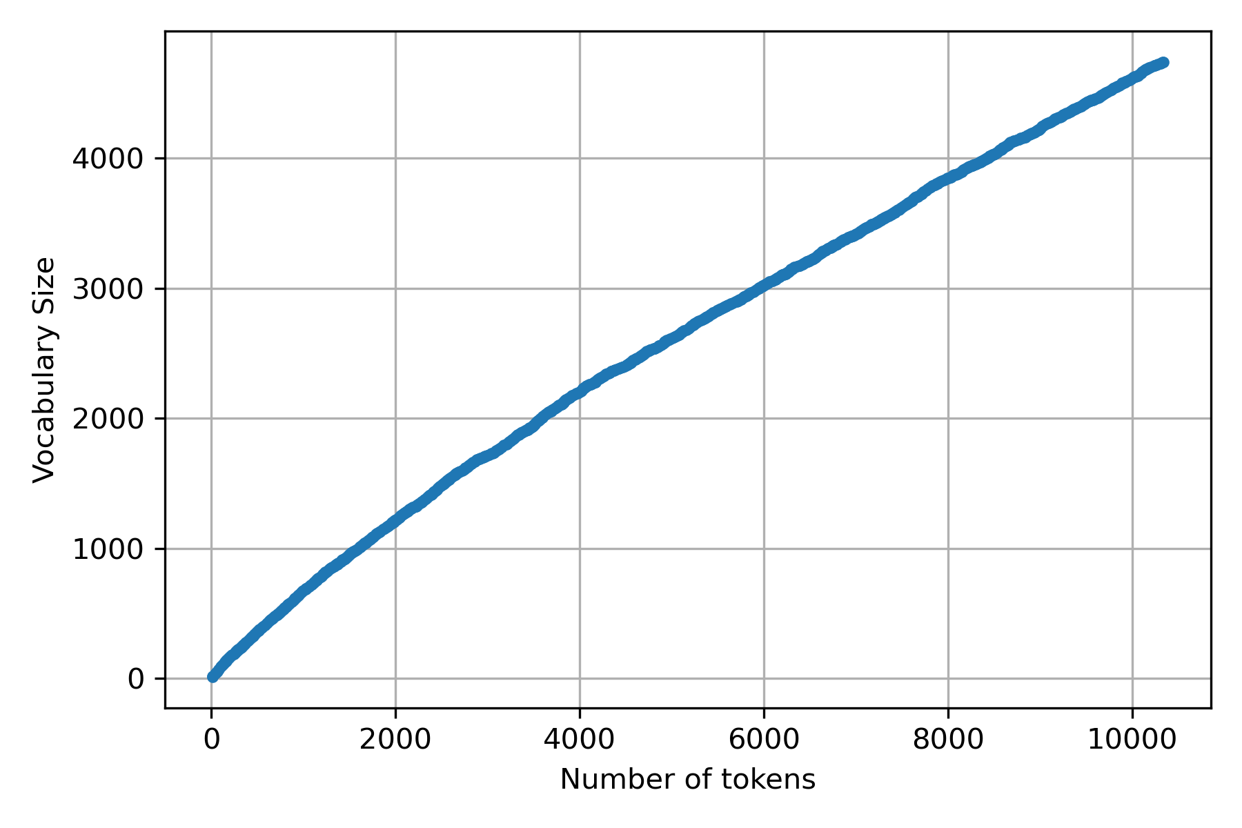
Taking the procedure used in Zipf’s Law as a starting point, it is only needed to collect, for each line, the number of words and the vocabulary.
words = Counter()
tokens_voc= list()
for tw in tweet_iterator(TWEETS):
    text = tw['text']
    words.update([x.strip() for x in text.split()])
    tokens_voc.append([sum(list(words.values())),
                       len(words)])

n = [x[0] for x in tokens_voc]
v = [x[1] for x in tokens_voc]
Once the points (number of words and vocabulary size) are measured, it is time to estimate the parameters \(k\) and \(\beta\). As can be observed, it is not possible to express the Heaps’ Law as a system of equations such as \(A \cdot [k, \beta]^\intercal = \mid \mathbf v \mid\); consequently, these parameters cannot be estimated using OLS.
Optimization
The values of these parameters can be estimated by posing them as an optimization problem. An optimization problem minimizes (maximizes) an objective function. The goal is to find the inputs corresponding to the minimum (maximum) of the function, i.e.,
\[\min_{\mathbf w \in \Omega} f(\mathbf w),\]where \(\mathbf w\) are the inputs of the function \(f\), and \(\Omega\) is the search space, namely the set containing all feasible values of the inputs, e.g., \(\Omega = \{\mathbf w \mid \mathbf w \in \mathbb R^d, \forall_i \mathbf w_i \geq 0\}\) that represents all the vector of dimension \(d\) whose components are equal or greater than zero.
There are many optimization algorithms; some are designed to tackle all possible optimization problems, and others are tailored for a particular class of problems. For example, OLS is an optimization algorithm where the objective function \(f\) is defined as:
\[f(\mathbf w) = \sum_{i=1}^N (y_i - \mathbf a_i \cdot \mathbf w)^2,\]where \(\mathbf w\) is a vector containing the parameters, and \(\mathbf a_i\) is the \(i\)-th measurement of the independent variables, and \(y_i\) is the corresponding dependent variable. In the Zipf’s Law example, \(\mathbf w\) corresponds to the parameter \(c\), \(\mathbf a_i\) is the \(i\)-the measure of the inverse rank, and \(y_i\) is the corresponding frequency.
Let us analyze in more detail the previous objective function. The sum goes for all the measurements; there are \(N\) pairs of observations composed by the response (dependent variable) and the independent variables. For each observation \(i\), the square error is computed between the dependent variable (\(y_i\)) and the dot product of the independent variable (\(\mathbf a_i\)) and parameters (\(\mathbf x\)).
This notation is specific for OLS; however, it is helpful to define the general case. The first step is to define the set \(\mathcal D\) composed by the \(N\) observations, i.e., \(\mathcal D=\{(\mathbf x_i, y_i) \mid 1 \leq i \leq N\}\) where \(y_i\) is the response variable and \(\mathbf x\) contains the independent variables. The second step is to use an unspecified loss function as \(L(y, \hat y) = (y - \hat y)^2\). The last step is to abstract the model, that is replace \(\mathbf a_i \cdot \mathbf w\) with a function \(g(\mathbf x) = \mathbf a_i \cdot \mathbf w\). Combining these components the general version of the OLS optimization problem can be expressed as:
where \(g\) are all the functions defined in the search space \(\Omega\), \(L\) is a loss function, and \(\mathcal D\) contains \(N\) pairs of observations. This optimization problem is known as supervised learning in machine learning.
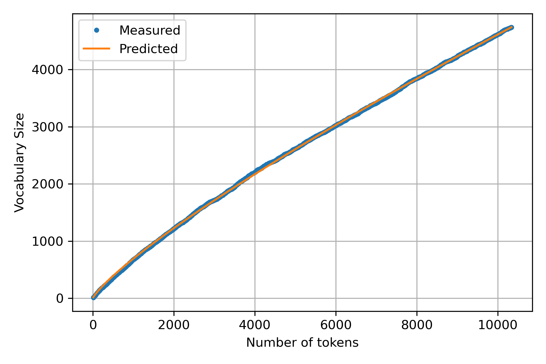
Returning to Heaps’ Law problem where the goal is to identify the coefficients \(k\) and \(\beta\) of the model \(\mid v \mid = kn^\beta\). That is, function \(g\) can be defined as \(g_{k,\alpha}(n) = kn^\beta\) and using the square error as \(L\) the optimization problem is:
\[\min_{(k, \beta) \in \mathbb R^2} \sum_{(n, \mid v \mid) \in \mathcal D} (\mid v \mid - kn^\beta)^2.\]As mentioned previously, there are many optimization algorithms; some can be found on the function scipy.optimize.minimize. The function admits as arguments the objective function and the initial values of the parameters.
The following code solves the optimization problem using the minimize function.
def f(w, y, x):
    k, beta = w
    return ((y - k * x**beta)**2).sum()

n = np.array(n)
v = np.array(v)
res = minimize(f, np.array([1, 0.5]), (v, n))
k, beta = res.x
k, beta
(2.351980550243793, 0.8231559504194587)
Once \(k\) and \(\beta\) have been identified, it is possible to use them in the Heaps’ Law and produce a figure containing the measurements and predicted values.
Activities
Zipf’s Law and Heaps’ Law model two language characteristics; these characteristics are summarized in the values of the parameters \(c\) and \(k\) and \(\beta\) respectively. So far, we have identified these parameters using a toy dataset. In order to illustrate how these parameters can be used to compare languages, we are going to use a dataset of words (and bi-grams) available in a library text_models described in A Python library for exploratory data analysis on twitter data based on tokens and aggregated origin–destination information.
text_models contains the frequency of words and bigrams of words measured from tweets written in different languages (Arabic, Spanish, and English) and collected from the Twitter open stream.
The first step is to retrieve the information from a particular date, location, and language. As an example, let us retrieve the data corresponding to January 10, 2022, in Mexico and written in Spanish, which can be done with the following code.
date = dict(year=2022, month=1, day=10)
voc = Vocabulary(date, lang='Es', country='MX')
words = {k: v for k, v in voc.voc.items() if not k.count('~')}
Variable voc contains the frequency of the words and bigrams and some useful functions to distill the information and perform an exploratory data analysis on the data. The raw data is stored in a dictionary on the variable voc.voc. The bi-grams are identified with the character ‘~’, e.g., ‘of~the’ corresponds to the bi-gram of the words of and the. Finally, the variable words contains the frequency of the words.
A traditional approach to explore the information of a list of words and their frequencies is to create a word cloud. The following figure is the word cloud of the frequency of the words retrieved from text_models.
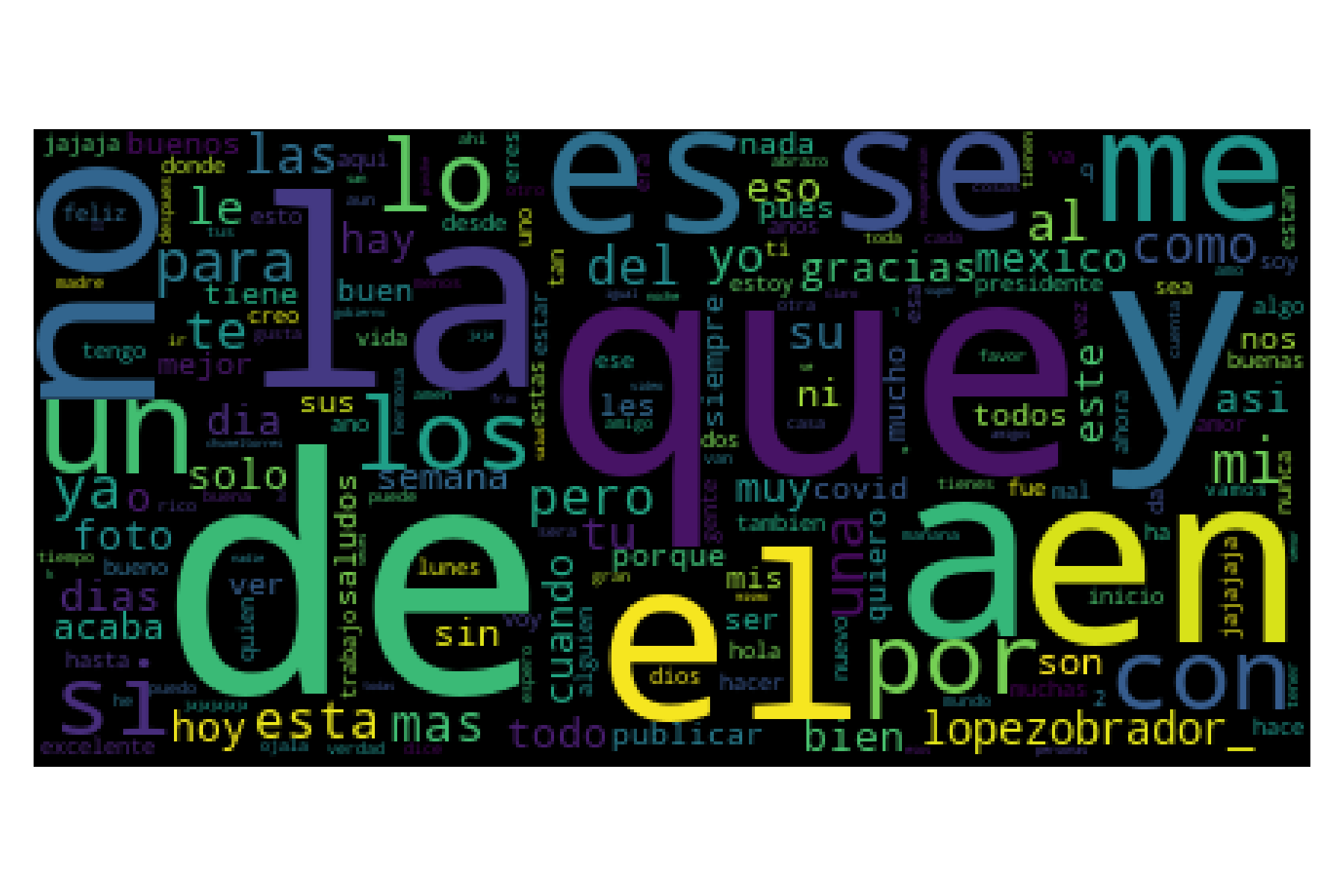
Code of the word cloud
wc = WC().generate_from_frequencies(words)
plt.imshow(wc)
plt.axis('off')
plt.tight_layout()
Zipf’s Law - \(f=\frac{c}{r}\)
We are in the position to identify the Zips’ Law coefficient from a dataset retrieved from text_models. In this part, the goal is to estimate \(c\) from all the Spanish-speaking countries on a particular date, January 10, 2022. On this occasion, the library joblib is used to parallelize the code, particularly the class Parallel. As can be seen, the variable words is a list of dictionaries containing the words frequency for all the countries.
countries = ['MX', 'CO', 'ES', 'AR',
             'PE', 'VE', 'CL', 'EC',
             'GT', 'CU', 'BO', 'DO',
             'HN', 'PY', 'SV', 'NI',
             'CR', 'PA', 'UY']
vocs = Parallel(n_jobs=-1)(delayed(Vocabulary)(date,
                                               lang='Es',
                                               country=country)
                               for country in tqdm(countries))
words = [{k: v for k, v in voc.voc.items() if not k.count('~')}
         for voc in vocs]
The next step is to estimate the \(c\) coefficient of Zipf’s Law. Function zipf identifies the coefficient using OLS from a dictionary of words frequency. Variable zipf_c contains the coefficient values for each country, and we also computed the number of words seen, which is stored in variable tokens.
def zipf(data):
    freq = [f for _, f  in Counter(data).most_common()]
    rank = 1 / np.arange(1, len(freq) + 1)
    X = np.atleast_2d(rank).T
    return np.linalg.lstsq(X, freq, rcond=None)[0]

zipf_c = [zipf(w) for w in words]
tokens = [sum(list(w.values())) for w in words]
The following table presents the coefficient \(c\) and the number of words (\(n\)) for all the countries. The table is sorted by \(c\) in descending order. It can be seen that \(c\) and \(n\) are highly correlated, so this version of Zipf’s Law only characterizes the total number of words seen on the dataset.
| Country | \(c\) | \(n\) |
|---|---|---|
| AR | 28383.27 | 405802 |
| ES | 21392.39 | 267724 |
| MX | 20166.90 | 269211 |
| CO | 11549.12 | 153952 |
| CL | 8324.78 | 114394 |
| VE | 4704.40 | 56019 |
| UY | 3714.85 | 52058 |
| PE | 2996.51 | 39945 |
| EC | 2768.21 | 35822 |
| PY | 1914.56 | 24544 |
| DO | 1843.01 | 22969 |
| PA | 1575.23 | 20726 |
| GT | 1312.07 | 17237 |
| NI | 756.56 | 8967 |
| HN | 704.90 | 8243 |
| CR | 607.04 | 6994 |
| CU | 604.96 | 6989 |
| SV | 513.01 | 5703 |
| BO | 416.46 | 4306 |
The following table shows the correlation of \(c\) and \(n\); it is observed that the correlation between them is higher than \(0.99\), this means that measuring the number of words is enough and there is no need to estimate \(c\).
| \(c\) | \(n\) | |
|---|---|---|
| \(c\) | 1.0000 | 0.9979 |
| \(n\) | 0.9979 | 1.0000 |
The correlation is obtained using the following code.
X = np.array([(b[0], c) for b, c in zip(zipf_c, tokens)])
corr = np.corrcoef(X.T)
Zipf’s Law - \(f=\frac{c}{r^\alpha}\)
Zipf’s Law has different versions; we started with the simpler one; however, that version does not provide information that the one contained in the number of words. A straightforward approach is to change the constant in Zipf’s Law with a parameter and then use an algorithm to estimate that constant. Zipf’s Law has the following form \(f=\frac{c}{r^1}\), where the constant is \(1\); changing \(1\) by \(\alpha\) it is obtained \(f=\frac{c}{r^\alpha}\). Without considering the meaning of the variables on this later version of Zipf’s Law, one can see the similarities between Zipf’s Law and Heap’s Law formulation; both have a multiplying constant \(c\) and \(k\), and an exponential one \(\alpha\) and \(\beta\).
Coefficients \(c\) and \(\alpha\) can be estimated using the dataset stored in variable words, the procedure is a combination of the approach used to identify \(c\) in the previous formulation and the algorithm described to estimate \(k\) and \(\beta\) of the Heap’s Law.
The following table shows the values of the coefficients \(c\), \(\alpha\), and the number of words for the different countries.
| Country | \(c\) | \(\alpha\) | \(n\) |
|---|---|---|---|
| AR | 24606.53 | 0.7627 | 405802 |
| MX | 17533.38 | 0.7715 | 269211 |
| ES | 18745.24 | 0.7842 | 267724 |
| CO | 10027.21 | 0.7691 | 153952 |
| CL | 7231.78 | 0.7716 | 114394 |
| VE | 4075.39 | 0.7695 | 56019 |
| UY | 3175.76 | 0.7432 | 52058 |
| PE | 2592.78 | 0.7690 | 39945 |
| EC | 2391.38 | 0.7672 | 35822 |
| PY | 1636.43 | 0.7488 | 24544 |
| DO | 1570.40 | 0.7425 | 22969 |
| PA | 1347.33 | 0.7514 | 20726 |
| GT | 1114.08 | 0.7408 | 17237 |
| NI | 645.04 | 0.7541 | 8967 |
| HN | 596.58 | 0.7379 | 8243 |
| CR | 512.80 | 0.7349 | 6994 |
| CU | 514.40 | 0.7470 | 6989 |
| SV | 435.75 | 0.7460 | 5703 |
| BO | 352.77 | 0.7409 | 4306 |
The correlation of these variables can be seen in the following table. It is observed that \(c\) is highly correlated with the number of words \(n\). On the other hand, the correlation between \(\alpha\) and \(n\) indicates that these variables contain different information.
| \(c\) | \(\alpha\) | \(n\) | |
|---|---|---|---|
| \(c\) | 1.0000 | 0.6588 | 0.9975 |
| \(\alpha\) | 0.6588 | 1.0000 | 0.6308 |
| \(n\) | 0.9975 | 0.6308 | 1.0000 |
Heaps’ Law - \(\mid v \mid = kn^\beta\)
Heaps’ Law models the relationship between the number of words (\(n\)) and the size of the vocabulary \(\mid v \mid\). In order to estimate the parameters, it is needed to obtain a dataset where \(n\) is varied and for each one compute \(\mid v \mid\). The dataset used to estimate the coefficients of Zipf’s Law contains \(n\) and \(\mid v \mid\) for a particular date, country, and language. \(\mid v \mid\) corresponds to the length of the dictionary, that is, the number of different words, namely the number for keys in it. Consequently, the dataset needed to estimate the coefficients of Heap’s Law can be obtained by collecting measuring \(n\) and \(\mid v \mid\) on different days.
The dataset can be obtained by first creating a helper function that contains the code used to retrieve the words in the function get_words.
COUNTRIES = ['MX', 'CO', 'ES', 'AR',
             'PE', 'VE', 'CL', 'EC',
             'GT', 'CU', 'BO', 'DO',
             'HN', 'PY', 'SV', 'NI',
             'CR', 'PA', 'UY']

def get_words(date=dict(year=2022, month=1, day=10)):


    vocs = Parallel(n_jobs=-1)(delayed(Vocabulary)(date,
                                                   lang='Es',
                                                   country=country)
                                   for country in tqdm(COUNTRIES))
    words = [{k: v for k, v in voc.voc.items() if not k.count('~')}
             for voc in vocs]
    return words
Function get_words retrieves the words for all the countries on a particular date; consequently, the next step is to decide the dates to create the dataset. The following code uses the function date_range to create a list of dates starting from November 1, 2021, and finishing on November 30, 2021 (inclusive). Variable words is a list where each element corresponds to a different day containing the words frequency of all the countries; however, to estimate the coefficients, it is needed to have a dataset for each country with all the days. The last line created the desired dataset; it is a list where each element has the frequency of the words for all the days of a particular country.
init = dict(year=2021, month=11, day=1)
end = dict(year=2021, month=11, day=30)
dates = date_range(init, end)
words = [get_words(d) for d in dates]
ww = [[w[index] for w in words] for index in range(len(COUNTRIES))]
The information stored in variable ww contains, for each country, the information needed to create \(n\) and \(\mid v \mid\). Function voc_tokens computes \(n\) and \(\mid v \mid\) for the dataset given, i.e., an element of ww. It uses the variable cnt as an accumulator; it is observed that the pattern of line 3 is used every time cnt is updated.
def voc_tokens(data):
    cnt = Counter(data[0])
    output = [[len(cnt), sum(list(cnt.values()))]]
    for x in data[1:]:
        cnt.update(x)
        _ = [len(cnt), sum(list(cnt.values()))]
        output.append(_)
    output = np.array(output)
    return output[:, 0], output[:, 1]
For example, voc_tokens can be used to create \(n\) and \(\mid v \mid\) of Mexico as:
n_mx, v_mx = voc_tokens(ww[0])
Having described how to obtain \(n\) and \(\mid v \mid\) for each country, it is time to use the procedure to estimate the country’s \(k\) and \(\beta\) coefficients. The following table shows the values of these coefficients for each country; it also includes the maximum number of words (\(\max n\)) in the last column.
| Country | \(k\) | \(\beta\) | \(\max n\) |
|---|---|---|---|
| AR | 10.19 | 0.5262 | 12883620 |
| ES | 2.40 | 0.6316 | 10495462 |
| MX | 4.79 | 0.5749 | 9738471 |
| CO | 8.31 | 0.5311 | 5987400 |
| CL | 11.13 | 0.5199 | 5689730 |
| UY | 10.68 | 0.5085 | 1659338 |
| EC | 7.46 | 0.5319 | 1491032 |
| VE | 4.20 | 0.5651 | 1387172 |
| PE | 11.09 | 0.5090 | 1249352 |
| PY | 9.28 | 0.5091 | 969505 |
| PA | 8.49 | 0.5209 | 885552 |
| DO | 6.15 | 0.5322 | 749857 |
| GT | 8.01 | 0.5135 | 556313 |
| HN | 4.94 | 0.5445 | 422616 |
| CU | 4.78 | 0.5611 | 305530 |
| NI | 9.15 | 0.4918 | 243830 |
| SV | 3.35 | 0.5703 | 240215 |
| CR | 5.71 | 0.5276 | 223434 |
| BO | 2.55 | 0.5958 | 159700 |
As we have seen previously, the correlation between the variables displays the relation between the coefficients; it was helpful to realize that the first version of Zipf’s Law was not needed. The following table shows the correlation between \(k\), \(\beta\), and \(\max n\). It is observed that \(k\) and \(\beta\) are uncorrelated to \(\max n\), and that there is a negative correlation between \(k\) and \(\beta\).
| \(k\) | \(\beta\) | \(\max n\) | |
|---|---|---|---|
| \(k\) | 1.0000 | -0.8643 | 0.0587 |
| \(\beta\) | -0.8643 | 1.0000 | 0.3235 |
| \(\max n\) | 0.0587 | 0.3235 | 1.0000 |
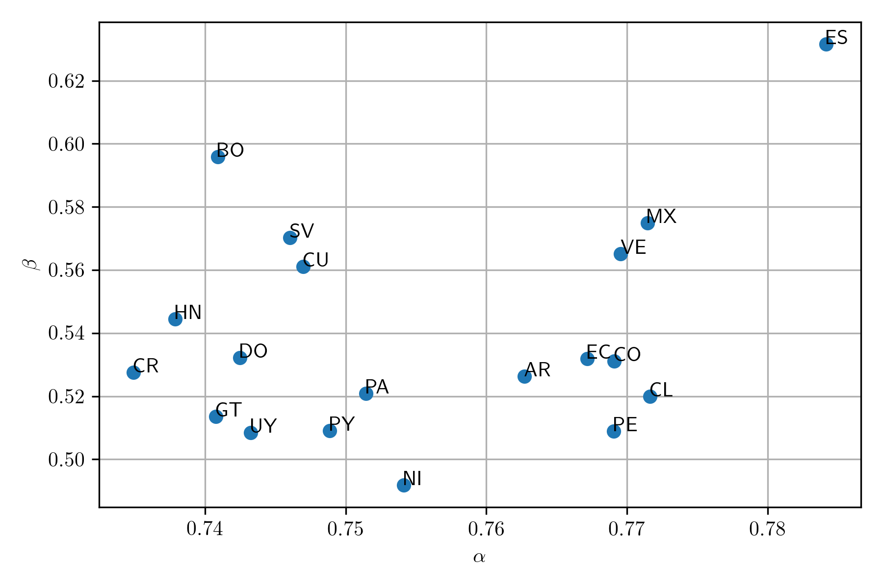
Comparison of Spanish-speaking countries
Coefficients \(\alpha\) and \(\beta\) characterize the vocabulary on a particular region, language, and dates. These coefficients can be used to compare the similarities between the countries. A simple approach is to create a scatter problem between \(\alpha\) and \(\beta\). The following figure shows the scatter plot of the Spanish-speaking countries.