Text Categorization (Vectors)
Contents
- Introduction
- Maximum Likelihood Estimator
- Text Categorization - Logistic Regression
- Lab: Bag of Words Text Categorization
Libraries used
import numpy as np
from b4msa.textmodel import TextModel
from EvoMSA.tests.test_base import TWEETS
from microtc.utils import tweet_iterator
from EvoMSA.utils import LabelEncoderWrapper, bootstrap_confidence_interval
from EvoMSA.model import Multinomial
from EvoMSA import BoW
from sklearn.model_selection import StratifiedKFold
from sklearn.linear_model import LogisticRegression
from sklearn.svm import LinearSVC
Installing external libraries
pip install b4msa
pip install evomsa
Introduction
The problem of text categorization can be tackled directly by modeling the conditional probability, i.e., \(\mathbb P(\mathcal Y=k \mid \mathcal X=x)=f_k(x)\) where \(f_k\) is the \(k\)-th value of \(f: \mathcal X \rightarrow [0, 1]^K\) which encodes a probability mass function. For the case of \(K\) classes an adequate distribution is Categorical, where function \(f\) takes the place of the parameter of the distribution, that is, \(\mathcal Y \sim \textsf{Categorical}(f(\mathcal X))\).
The parameters of the function \(f\) can be identified using a maximum likelihood estimator; this procedure is equivalent to the one used for parameter \(\mathbf p\) of the Categorical distribution.
Maximum Likelihood Estimator
The log-likelihood estimator is defined as follows, where \(\mathcal D\) is the dataset used to estimate the parameters, \(f_\mathcal Y\) is the probability mass function that corresponds to the Categorical distribution, and \(f(x)\) takes the place of the distribution parameter; as can be observed, it is a function of the input.
\[\begin{eqnarray} l_{f_\mathcal Y}(f) &=& \log \prod_{(x, y) \in \mathcal D} f_\mathcal Y(y \mid f(x)) \\ &=& \log \prod_{(x, y) \in \mathcal D} \prod_{k=1}^K f_k(x)^{\mathbb 1(k=y)}\\ \end{eqnarray}\]Assuming that function \(f\) has a parameter \(w_j\), the procedure to estimate the parameter is to compute the partial derivate of the log-likelihood with respect to \(w_j\) and solve it when it is equal to zero.
\[\begin{eqnarray} \frac{\partial}{\partial w_j} l_{f_\mathcal Y}(f) &=& \frac{\partial}{\partial w_j} \log \prod_{(x, y) \in \mathcal D} \prod_{k=1}^K f_k(x)^{\mathbb 1(k=y)}\\ &=& \frac{\partial}{\partial w_j} \sum_{(x, y) \in \mathcal D} \sum_{k=1}^K \mathbb 1(k=y) \log f_k(x) = 0 \end{eqnarray}\]Minimizing Cross-entropy
Before solving the log-likelihood, it is essential to relate this concept with cross-entropy. First the expectation of \(h(\mathcal X)\) is computed as \(\sum_{k \in \mathcal X} h(k) f(k)\) where \(f\) is the mass function, this can be expressed as \(\mathbb E_f[h(\mathcal X)]\). On the other hand, the information content of an event is a decreasing function that has its zero when the event has the highest probability, meaning that there is no information carried on an event that occurs always. The information content can be modeled with the function \(I_f(e) = \log(\frac{1}{f(e)})=-\log(f(e)).\) The entropy measures the expected value of the information content that is \(\mathbb E_f[I_f(\mathcal X)]=-\sum_{k \in \mathcal X} f(k) \log(f(k)).\) Finally, the cross-entropy between distribution \(p\) and \(q\) is defined as \(H(p, q) = \mathbb E_p[I_q(\mathcal X)] = -\sum_{k \in \mathcal X} p(k) \log(q(k)).\)
It can be observed that the negative of the log-likelihood is accumulating the cross-entropy for all the elements in the dataset \(\mathcal D\), i.e., probability \(p(k)\) is \(\mathbb 1(y=k)\), and \(q(k)=f_k(x)\) using the previous definition of cross-entropy \(H(p, q)\). The characteristic to note is that \(y\) and \(x\) are constants in the inner summation, and variable \(k\) goes from all the classes. Therefore, minimizing the log-likelihood is minimizing the cross-entropy, which acts as the loss function \(L\) in the optimization problem.
\[\begin{eqnarray} -\frac{\partial}{\partial w_j} l_{f_\mathcal Y}(f) &=& \frac{\partial}{\partial w_j} \sum_{(x, y) \in \mathcal D} \overbrace{- \sum_{k=1}^K \mathbb 1(k=y) \log f_k(x)}^{cross-entropy} \\ &=& -\sum_{(x, y) \in \mathcal D} \sum_{k=1}^K \mathbb 1(k=y) \frac{\partial}{\partial w_j} \log f_k(x)\\ &=& - \sum_{(x, y) \in \mathcal D} \sum_{k=1}^K \frac{\mathbb 1(k=y)}{f_k(x)} \frac{\partial}{\partial w_j} f_k(x) \end{eqnarray}\]The function \(f_k\) has a constraint given that it is taking the place of parameter \(\mathbf p\) of the Categorical Distribution; this restriction is \(\sum_k^K f_k(x) = 1\) which can be complied by dividing it with a normalization factor as:
\[f_k(x) = \frac{h_k(w_k(x))}{\sum_{\ell=1}^K h_\ell(w_\ell(x))}\]The next step is to compute the partial derivative with respect to \(w_j\)
\[\begin{eqnarray} \frac{\partial}{\partial w_j} f_k(x) &=& \frac{\partial}{\partial w_j} \frac{h_k(w_k(x))}{\sum_{\ell=1}^K h_\ell(w_\ell(x))}\\ &=& \frac{\sum_{\ell=1}^K h_\ell(w_\ell(x)) \frac{\partial}{\partial w_j} h_k(w_k(x)) - h_k(w_k(x)) \frac{\partial}{\partial w_j} \sum_{\ell=1}^K h_\ell(w_\ell(x))}{(\sum_{\ell=1}^K h_\ell(w_\ell(x)))^2}\\ &=& \frac{\sum_{\ell=1}^K h_\ell(w_\ell(x)) \frac{\partial}{\partial w_j} h_k(w_k(x)) - h_k(w_k(x)) \frac{\partial}{\partial w_j} h_j(w_j(x))}{(\sum_{\ell=1}^K h_\ell(w_\ell(x)))^2}. \end{eqnarray}\]Substituting the partial derivative of \(f_k\) into the negative log-likelihood is obtained
\[\begin{eqnarray} -\frac{\partial}{\partial w_j} l_{f_\mathcal Y}(f) &=& - \sum_{(x, y) \in \mathcal D} \sum_{k=1}^K \frac{\mathbb 1(k=y)}{f_k(x)} \frac{\partial}{\partial w_j} f_k(x)\\ &=& - \sum_{(x, y) \in \mathcal D} \sum_{k=1}^K \frac{\mathbb 1(k=y)}{h_k(w_k(x))} \frac{\sum_{\ell=1}^K h_\ell(w_\ell(x)) \frac{\partial}{\partial w_j} h_k(w_k(x)) - h_k(w_k(x)) \frac{\partial}{\partial w_j} h_j(w_j(x))}{\sum_{\ell=1}^K h_\ell(w_\ell(x))} \end{eqnarray}\]Multinomial Logistic Regression
In order to progress with derivation, it is needed to make some assumptions; the assumption that produce the Multinomial Logistic Regression algorithm is that \(h_k\) is the exponent, i.e., \(h_k(x)= \exp(x)\) and the resulting \(f_k\) is the softmax function.
\[\begin{eqnarray} h_k(w_k(x)) &=& \exp(w_k(x))\\ f_k(w_k(x)) &=& \frac{\exp(w_k(x))}{\sum_\ell \exp(w_\ell(x))} \end{eqnarray}\]Using \(f_k\) as the softmax function in the negative log-likelihood produces the following
\[\begin{eqnarray} -\frac{\partial}{\partial w_j} l_{f_\mathcal Y}(f) &=& - \sum_{(x, y) \in \mathcal D} \sum_{k=1}^K \frac{\mathbb 1(k=y)}{\exp(w_k(x))} \frac{\sum_{\ell=1}^K \exp(w_\ell(x)) \frac{\partial}{\partial w_j} \exp(w_k(x)) - \exp(w_k(x)) \exp(w_j(x)) \frac{\partial}{\partial w_j} w_j(x)}{\sum_{\ell=1}^K \exp(w_\ell(x))}\\ &=& - \sum_{(x, y) \in \mathcal D} \sum_{k=1}^K \frac{\mathbb 1(k=y)}{\exp(w_k(x))} \frac{\sum_{\ell=1}^K \exp(w_\ell(x)) \exp(w_k(x)) \frac{\partial}{\partial w_j} w_k(x) - \exp(w_k(x)) \exp(w_j(x)) \frac{\partial}{\partial w_j} w_j(x)}{\sum_{\ell=1}^K \exp(w_\ell(x))}\\ &=& - \sum_{(x, y) \in \mathcal D} \sum_{k=1}^K \mathbb 1(k=y) \frac{\sum_{\ell=1}^K \exp(w_\ell(x)) \frac{\partial}{\partial w_j} w_k(x) - \exp(w_j(x)) \frac{\partial}{\partial w_j} w_j(x)}{\sum_{\ell=1}^K \exp(w_\ell(x))}\\ &=& - \sum_{(x, y) \in \mathcal D} \sum_{k=1}^K \mathbb 1(k=y) \left[ \frac{\partial}{\partial w_j} w_k(x) - f_j(w_j(x)) \frac{\partial}{\partial w_j} w_j(x)\right]\\ &=& - \sum_{(x, y) \in \mathcal D} \mathbb 1(j=y) \left[ \frac{\partial}{\partial w_j} w_j(x) - f_j(w_j(x)) \frac{\partial}{\partial w_j} w_j(x)\right] + \sum_{k \neq j}^K \mathbb 1(k=y) \left[ \frac{\partial}{\partial w_j} w_k(x) - f_j(w_j(x)) \frac{\partial}{\partial w_j} w_j(x)\right]\\ &=& - \sum_{(x, y) \in \mathcal D} \mathbb 1(j=y) \left[ 1 - f_j(w_j(x)) \right] \frac{\partial}{\partial w_j} w_j(x) + \sum_{k \neq j}^K -\mathbb 1(k=y) f_j(w_j(x)) \frac{\partial}{\partial w_j} w_j(x)\\ &=& - \sum_{(x, y) \in \mathcal D} \left( \mathbb 1(j=y) - f_j(w_j(x)) \right) \frac{\partial}{\partial w_j} w_j(x)\\ &=& \sum_{(x, y) \in \mathcal D} \left( f_j(w_j(x)) - \mathbb 1(j=y) \right) \frac{\partial}{\partial w_j} w_j(x). \end{eqnarray}\]Logistic Regression
On the other hand, the Logistic Regression algorithm is obtained when one assumes that \(f_1\) is the sigmoid function and there are two classes; furthermore, this assumption makes it possible to express \(f_2\) in terms of \(f_1\) as follows:
\[\begin{eqnarray} f(x) &=& \frac{1}{1 + \exp(-x)}\\ f_1(x) &=& f(w(x)) \\ f_2(x) &=& 1 - f_1(x). \end{eqnarray}\]Using \(f_1\), \(f_2\), and the sigmoid function in the negative log-likelihood produce the following
\[\begin{eqnarray} -\frac{\partial}{\partial w_j} l_{f_\mathcal Y}(f) &=& - \sum_{(x, y) \in \mathcal D} \sum_{k=1}^K \frac{\mathbb 1(k=y)}{f_k(x)} \frac{\partial}{\partial w_j} f_k(x)\\ &=& - \sum_{(x, y) \in \mathcal D} \frac{\mathbb 1(1=y)}{f_1(x)} \frac{\partial}{\partial w_j} f_1(x) + \frac{\mathbb 1(2=y)}{1 - f_1(x)} \frac{\partial}{\partial w_j} \left( 1 - f_1(x) \right)\\ &=& - \sum_{(x, y) \in \mathcal D} \frac{\mathbb 1(1=y)}{f(w(x))} \frac{\partial}{\partial w_j} f(w(x)) - \frac{\mathbb 1(2=y)}{1 - f(w(x))} \frac{\partial}{\partial w_j} f(w(x))\\ &=& - \sum_{(x, y) \in \mathcal D} \left[ \frac{\mathbb 1(1=y)}{f(w(x))} - \frac{\mathbb 1(2=y)}{1 - f(w(x))} \right] \frac{\partial}{\partial w_j} f(w(x))\\ &=& - \sum_{(x, y) \in \mathcal D} \left[ \frac{\mathbb 1(1=y)}{f(w(x))} - \frac{\mathbb 1(2=y)}{1 - f(w(x))} \right] (1 - f(w(x))) f(w(x)) \frac{\partial}{\partial w_j} w(x)\\ &=& - \sum_{(x, y) \in \mathcal D} \left[ (1 - f(w(x)))\mathbb 1(1=y) - f(w(x))\mathbb 1(2=y) \right] \frac{\partial}{\partial w_j} w(x)\\ &=& - \sum_{(x, y) \in \mathcal D} (\mathbb 1(1=y) - f(w(x))) \frac{\partial}{\partial w_j} w(x)\\ &=& \sum_{(x, y) \in \mathcal D} (f(w(x)) - \mathbb 1(1=y)) \frac{\partial}{\partial w_j} w(x) \end{eqnarray}.\]It can be observed that the form of the negative log-likelihood for the Multinomial Logistic Regression and the Logistic Regression is similar; the only difference is that there is a function \(w\) for each class in the multinomial case, and only one function for the Logistic Regression.
Text Categorization - Logistic Regression
Additionally, there has been no assumption regarding the form of \(w(x)\); given that the problem is text categorization, the variable \(x\) corresponds to a text. However, the standard definition of Multinomial Logistic Regression and Logistic Regression is that function \(w\) is a linear function, i.e., \(w(x) = \mathbf w \cdot \mathbf x + w_0\) where \(\mathbf w \in \mathbb R^d\), \(\mathbf x \in \mathbb R^d\), and \(w_0 \in \mathbb R\). Consequently, one needs to define a function \(m: text \rightarrow \mathbb R^d\) so that \(m(x) \in \mathbb R^d\); the Multinomial Logistic Regression in this problem turns out to be:
\[\mathbb P(\mathcal Y=k \mid \mathcal X=x) = \frac{\exp(\mathbf w_k m(x) + w_{k_0})}{\sum_{j=1}^K \exp(\mathbf w_j m(x) + w_{k_0})}.\]The denominator in the previous equation acts as a normalization factor, and the predicted class is invariant to this normalization factor. Additionally, the logarithm of \(\mathbb P(\mathcal Y=k \mid \mathcal X=x)\) does not affect the prediction class with the rule \(\textsf{class(x)} = \textsf{arg max}_k \mathbb P(\mathcal Y=k \mid \mathcal X=x).\) Considering these factors the class is predicted as
\[\textsf{class(x)} = \textsf{arg max}_k \mathbf w_k m(x) + w_{k_0}.\]The first approach followed to tackle the problem of Text Categorization was to use the Bayes’ Theorem \((\mathbb P(\mathcal Y \mid \mathcal X) = \frac{\mathbb P(\mathcal X \mid \mathcal Y) \mathbb P(\mathcal Y)}{\mathbb P(\mathcal X)})\) where the likelihood (\(\mathbb P(\mathcal X \mid \mathcal Y)\)) is assumed to be a Categorical Distribution. A Categorical Distribution is defined with a vector \(\mathbf p \in \mathbb R^d\) where \(d\) is the different distribution outcomes. The likelihood is a Categorical Distribution given the class \(\mathcal Y\), therefore there is a parameter \(\mathbf p\) for each class, which can be identified with a subindex \(k\), e.g., \(\mathbf p_k\) is the parameter corresponding to the class \(k\). The parameters are estimated assumming indepedence, i.e., \(\mathbb P(\mathcal X=w_1,w_2,\ldots,w_\ell \mid \mathcal Y) = \prod_i^\ell \mathbb P(w_i \mid \mathcal Y),\) where \(w_i\) is the \(i\)-th token in the text.
The evidence \(\mathbb P(\mathcal X)\) is a normalization factor in Bayes’ theorem, so it does not affect the predicted class; moreover, the logarithm does not change the prediction value. Incorporating into Bayes’ theorem these transformations, it is obtained
\[\log \mathbb P(\mathcal Y \mid \mathcal X=w_1,w_2,\ldots,w_\ell) \propto \sum_i^\ell \log \mathbb P(w_i \mid \mathcal Y) + \log \mathbb P(\mathcal Y);\]which can be expressed using the parameter, \(\mathbf p_k\), of the Categorical Distribution, and the frequency of each token as follows:
\[\log \mathbb P(\mathcal Y=k \mid \mathcal X=x) \propto \sum_i^d \log(\mathbf p_{k_i}) \textsf{freq}_i(x) + \log \mathbb P(\mathcal Y),\]where \(\textsf{freq}_i(x)\) computes the frequency of the token identified with the index \(i\) in the text \(x\). In order to illustrate the similarity between the previous equation and the one obtained with Multinomial Logistic Regression, it is convenient to express it using vectors, i.e., \(\log \mathbb P(\mathcal Y=k \mid \mathcal X=x) \propto \log(\mathbf p_k) \textsf{freq}(x) + \log P(\mathcal Y),\) where \(\log(\mathbf p_k) \in \mathbb R^d\), \(\textsf{freq}(x) \in \mathbb R^d\), and \(\log \mathbb P(\mathcal Y=k) \in \mathbb R.\) Therefore, the parameters \(\log(\mathbf p_k)\) and \(\log \mathbb P(\mathcal Y=k)\) are equivalent to \(\mathbf w\) and \(w_0\) in the (Multinomial) Logistic Regression, and \(m(x)\) is the frequency, \(\textsf{freq}(x)\), in the Categorical Distribution approach.
Gradient Descent Algorithm
The parameters \(\mathbf w\) and \(w_0\) can be estimated by minimizing the negative log-likelihood or equivalently by using the cross-entropy as loss function. Unfortunately, the system of equations \(-\frac{\partial}{\partial w_j} l_{f_\mathcal Y}(f) = 0\) cannot be solved analytically, so one needs to rely on numerical methods to find the \(w_j\) value that makes the function minimal. One approach that has been very popular lately is the gradient descent algorithm. The idea is that the parameter \(w_j\) can be found iterative using the update rule
\[w^i_j = w^{i-1}_j - \eta \frac{\partial}{\partial w_j} \sum_{(x, y) \in \mathcal D} L(y, g(x)).\]The Logistic Regression update rule is
\[w^i_j = w^{i-1}_j - \eta \sum_{(x, y) \in \mathcal D} (f(\mathbf w \cdot \mathbf x + w_0) - \mathbb 1(1=y)) \frac{\partial}{\partial w_j} \mathbf w \cdot \mathbf x + w_0,\]and the Multinomial Logistic Regression corresponds to
\[\mathbf w^i_{j_\ell} = \mathbf w^{i-1}_{j_\ell} - \eta \sum_{(x, y) \in \mathcal D} \left( f_j(\mathbf w_j \cdot \mathbf x + w_0) - \mathbb 1(j=y) \right) \frac{\partial}{\partial \mathbf w_{j_\ell}} \mathbf w_j \cdot \mathbf x + w_{j_0}.\]Term Frequency
Gradient descent algorithm is an option to estimate the parameters \(\mathbf w\) and \(w_0\) in (Multinomial) Logistic Regression and, in general, any algorithm that uses as its last step the sigmoid or softmax function. The missing step is to define the function \(m\); the approach that has been used in the Categorical Distribution is to use the frequency as \(m\).
The following code relies on the class TextModel to represent the text in a vector space, where the vector’s component is the frequency of each token of the input.
The following code reads a dataset and encodes the classes into unique identifiers; the first one is zero.
D = [(x['text'], x['klass']) for x in tweet_iterator(TWEETS)]
y = [y for _, y in D]
le = LabelEncoderWrapper().fit(y)
y = le.transform(y)
Once the dataset is in \(\mathcal D\), it can be used to train the class TextModel, which can be done with the method fit. The training is the process of associating each token with an id and identifying the size of the vocabulary in \(\mathcal D\).
tm = TextModel(token_list=[-1],
               weighting='tf').fit([x for x, _ in D])
The instance tm can be used to represent any text in the vector space; given that it is a sparse vector, it only outputs the dimensions where the value is different from zero, for example, the text buenos dias dias (good morning morning) is represented as:
vec = tm['buenos dias dias']
vec
[(263, 0.3333333333333333), (87, 0.6666666666666666)]
where the component identified as 263 (buenos) has the value of \(0.33\) and the component 87 (dias) is \(0.66\); the particular method’s characteristic is that the frequency is normalized.
The TextModel contains the transform method that can transform a list of texts into the vector space; the output of the method is a sparse matrix. The method can be used as follows.
X = tm.transform(['buenos dias dias'])
X.shape
(1, 3291)
The transform method can be combined with the implementation of Multinomial Logistic Regression of sklearn and tested under k-fold cross-validation to compute its performance in \(\mathcal D\).
folds = StratifiedKFold(shuffle=True, random_state=0)
hy = np.empty(len(D))
for tr, val in folds.split(D, y):
    _ = [D[x][0] for x in tr]
    X = tm.transform(_)
    m = LogisticRegression(multi_class='multinomial').fit(X, y[tr])
    _ = [D[x][0] for x in val]
    hy[val] = m.predict(tm.transform(_))
ci = bootstrap_confidence_interval(y, hy)
ci
(0.2839760475399691, 0.30881116416736665)
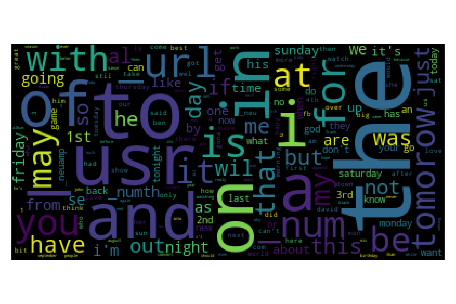
The following wordcloud shows the frequency in Semeval-2017 Task 4. It can be observed that the most frequent words are tokens that could be considered stopwords.
Term Frequency - Inverse Document Frequency
The term frequency is not the only weighting scheme available; one can develop different procedures that can be used to transform the text into a vector space. One of the most popular ones is the term frequency-inverse document frequency (tf-idf). The tf-idf is defined as the product of the term frequency, \(\textsf{tf}_i(x),\) and the inverse document frequency \(\textsf{idf}_i(x).\) The term frequency is defined as:
\[\textsf{tf}_i(x) = \frac{\sum_{w \in x} \mathbb 1(w = i)}{\mid x \mid},\]where \(x\) is the tokenized text represented as a multiset, using the identifiers instead of the token. On the other hand, the inverse document frequency is
\[\textsf{idf}_i(\mathcal D) = \log \frac{\mid \mathcal D \mid}{\sum_{x \in \mathcal D} \mathbb 1(i \in x) },\]where \(\mathcal D\) is the dataset used to train the algorithm and \(x\) is the tokenized text represented as a multiset.
The TextModel class uses as default weighting scheme tf-idf, which can be tested with the following code.
tm = TextModel(token_list=[-1]).fit([x for x, _ in D])
vec = tm['buenos dias']
vec
[(263, 0.7489370345067511), (87, 0.6626411686155892)]
The performance of this weighting scheme on \(\mathcal D\) can be estimated with the following code.
hy = np.empty(len(D))
for tr, val in folds.split(D, y):
    _ = [D[x][0] for x in tr]
    X = tm.transform(_)
    m = LogisticRegression(multi_class='multinomial').fit(X, y[tr])
    # m = LinearSVC().fit(X, y[tr])
    _ = [D[x][0] for x in val]
    hy[val] = m.predict(tm.transform(_))

ci = bootstrap_confidence_interval(y, hy)
ci
(0.31927898144547495, 0.34791512559623444)
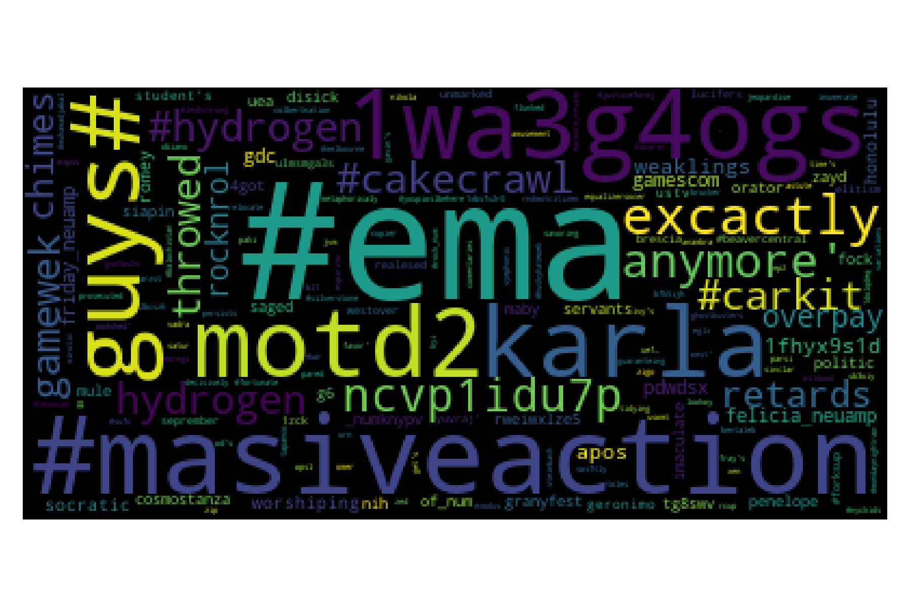
The inverse term frequency description is complemented by the word-cloud obtained with the Semeval-2017 Task 4 dataset. It can be seen that the words with the highest weights are infrequent.
Lab: Bag of Words Text Categorization
The previous section and this one have presented the elements to create a text classifier using a Bag of Words (BoW) representation (i.e., function \(m\) defined previously). It is time to wrap all this up and describe how to use Python’s class BoW that implements it.
The first step is to initialize the BoW representation; this can be done in two different ways. The first one is to use a pre-trained BoW representation which was trained in half a million tweets in each language available. The second is initializing the model with the data used to fit the text classifier.
The pre-trained BoW representation can be invoked, as shown in the following instruction.
bow = BoW(lang='en')
The instance bow can be used immediately because it uses a pre-trained model. The method transform receives a list of text to be transformed in the BoW representation; for example, the following code converts the text good morning into the representation.
bow.transform(['good morning'])
<1x16384 sparse matrix of type '<class 'numpy.float64'>'
	with 35 stored elements in Compressed Sparse Row format>
It is observed that the matrix has dimensions \(1 \times 16384\), which corresponds to one text, and the space is in \(\mathbb R^{16384}\) , meaning that there are \(16384\) tokens in the vocabulary. The matrix is in a sparse notation because only the tokens that appear in the text have a value other than zero.
The coefficients can be seen on the attribute data shown below.
X = bow.transform(['good morning'])
X.data
array([0.0418059 , 0.04938095, 0.06065429, 0.06554808, 0.07118364,
       0.07193482, 0.07464737, 0.07582207, 0.07998881, 0.08907673,
       0.1158131 , 0.1199745 , 0.12253494, 0.12477663, 0.13641194,
       0.13701824, 0.14673512, 0.17245292, 0.17909476, 0.18174817,
       0.18521041, 0.19004645, 0.19137817, 0.19414765, 0.19702447,
       0.20182253, 0.20188162, 0.20262674, 0.21067728, 0.24080574,
       0.24246672, 0.24981461, 0.26030563, 0.26209842, 0.27140846])
It can be observed that only 35 tokens have a value different than zero. These tokens correspond to the ones obtained from the text that are also in the representation’s vocabulary. BoW uses as a weighting scheme TF-IDF; however, all the vectors are normalized to be a unit vector, as can be verified in the previous example.
The non-zero tokens are stored in the attribute indices; however, these represent the index in the vector space. The attribute BoW.names has the actual token ordered equivalent to the vector space. The following code shows the tokens used to represent the text good morning.
' '.join([bow.names[x] for x in X.indices])
'q:in q:d~ q:~m q:ng q:or q:g~ q:ing q:ng~ q:ing~ q:~g q:oo q:ni q:mo q:go q:~go q:od q:~mo q:rn q:od~ q:ood q:mor q:nin q:ood~ q:ning q:goo q:~goo q:good q:~mor good q:orn q:rni q:rnin q:orni q:morn morning'
The second procedure to initialize the BoW class is using the same dataset to train the classifier; this approach is illustrated using a synthetic dataset found on the EvoMSA package. The dataset path is in the variable TWEETS and can be read using the tweet_iteration function, as shown in the following instructions.
D = list(tweet_iterator(TWEETS))
The BoW class is instantiated with the parameter pretrain set to false, as illustrated next.
bow = BoW(pretrain=False)
It can be verified that, at this time, it is impossible to transform any text into the BoW representations because the BoW model has yet to be trained.
The dataset in D is a Spanish polarity set with four positive, negative, neutral, and none labels. The text is in the keyword text, and the associate label is in the keyword klass; this can be changed and set to the appropriate values of the parameters key and labe_key of the BoW constructor.
D has all the components to train a text classifier; this can be done with the method fit. Internally, the method fit will invoke the method b4msa_fit to estimate the parameters of the BoW representation before training the classifier. The following code shows how to fit the text classifier.
bow.fit(D)
The variable bow can be used to predict the polarity of a given text; this can be done with the method predict. For example, the following code predicts the text buenos días (good morning).
bow.predict(['buenos dias'])
array(['P'], dtype='<U4')
The method predict receives a list of text, and it can be observed that the text buenos días is predicted as P, which corresponds to the positive class.