Text Categorization (Categorical Distribution)
Contents
- Introduction
- Bayes’ theorem
- Accuracy
- Confidence Interval
- Text Categorization - Categorical Distribution
- Performance
- Tokenizer
Libraries used
import numpy as np
from b4msa.textmodel import TextModel
from EvoMSA.tests.test_base import TWEETS
from microtc.utils import tweet_iterator, load_model, save_model
from scipy.stats import norm, multinomial, multivariate_normal
from matplotlib import pylab as plt
from collections import Counter
from sklearn.model_selection import StratifiedKFold
from scipy.special import logsumexp
from sklearn.metrics import recall_score, precision_score, f1_score
from EvoMSA.utils import bootstrap_confidence_interval
from sklearn.naive_bayes import MultinomialNB
from os.path import join
Installing external libraries
pip install b4msa
pip install evomsa
Introduction
Text Categorization is an NLP task that deals with creating algorithms capable of identifying the category of a text from a set of predefined categories. For example, sentiment analysis belongs to this task, and the aim is to detect the polarity (e.g., positive, neutral, or negative) of a text. Furthermore, different NLP tasks that initially seem unrelated to this problem can be formulated as a classification one such as question answering and sentence entailment, to mention a few.
Text Categorization can be tackled from different perspectives; the one followed here is to treat it as a supervised learning problem. As in any supervised learning problem, the starting point is a set of pairs, where the first element of the pair is the input and the second one corresponds to the output. Let \(\mathcal D = \{(\text{text}_i, y_i) \mid i=1,\ldots, N\}\) where \(y \in \{c_1, \ldots c_K\}\) and \(\text{text}_i\) is a text.
Supervised learning problems can be seen as finding a mapping function from inputs to outputs. The tool could be an optimization algorithm capable of finding the function that minimizes a particular loss function, e.g., \(L\).
\[\min_{g \in \Omega} \sum_{(\mathbf x, y) \in \mathcal D} L(y, g(\mathbf x)),\]where \(\Omega\) is the search space of the feasible mapping functions.
Additionally, if one is also interested in measuring the uncertainty, the path relies on probability. In this latter scenario, one approach is to assume the form of the conditional probability, i.e., \(\mathbb P(\mathcal Y=k \mid \mathcal X=x)=f_k(x)\) where \(f_k\) is the \(k\)-th value of \(f: \mathcal X \rightarrow [0, 1]^K\) which encodes a probability mass function. For the case of a binary classification problem the function is \(f: \mathcal X \rightarrow [0, 1]\). As can be seen, in this scenario, an adequate distribution is Bernoulli, where function \(f\) takes the place of the parameter of the distribution, that is, \(\mathcal Y \sim \textsf{Bernoulli}(f(\mathcal X))\); for more labels, the Categorical distribution can be used. On the other hand, the complement path is to rely on Bayes’ theorem.
Bayes’ theorem
The bivariate distribution \(\mathbb P(\mathcal X, \mathcal Y)\) can be expressed using the conditional probability as:
\[\begin{eqnarray} \mathbb P(\mathcal X, \mathcal Y) &=& \mathbb P(\mathcal X \mid \mathcal Y) \mathbb P(\mathcal Y)\\ \mathbb P(\mathcal X, \mathcal Y) &=& \mathbb P(\mathcal Y \mid \mathcal X) \mathbb P(\mathcal X). \end{eqnarray}\]These elements can be combined to obtain Bayes’ theorem following the next steps:
\[\begin{eqnarray} \mathbb P(\mathcal Y \mid \mathcal X) \mathbb P(\mathcal X) &=& \mathbb P(\mathcal X \mid \mathcal Y) \mathbb P(\mathcal Y)\\ \mathbb P(\mathcal Y \mid \mathcal X) &=& \frac{\mathbb P(\mathcal X \mid \mathcal Y) \mathbb P(\mathcal Y)}{\mathbb P(\mathcal X)}, \end{eqnarray}\]where \(\mathbb P(\mathcal Y \mid \mathcal X)\) is the posterior probability, \(\mathbb P(\mathcal X \mid \mathcal Y)\) corresponds to the likelihood, \(\mathbb P(\mathcal Y)\) is the prior, and \(\mathbb P(\mathcal X)\) is the evidence. The evidence can be expressed as \(\mathbb P(\mathcal X) = \sum_y \mathbb P(\mathcal X \mid \mathcal y) \mathbb P(\mathcal y)\) which corresponds to the marginal \(\mathbb P(\mathcal X)\) using the conditional probability; it can be observed that this term acts as a normalization constant.
The Bayes’ theorem has two features that make it amenable to addressing classification problems. The first is that it is a generative model; besides tackling the classification problem, the model can be used to generate the data, i.e., the model learns the distribution of the dataset.
The second characteristic is that the likelihood is a probability distribution given any class. Consequently, the problem is to estimate \(K\) different distribution using the subset of the training set belonging to each different class. On the other hand, the prior is the estimated probability of each class, and the evidence can be estimated using the previous two values.
Normal Distribution
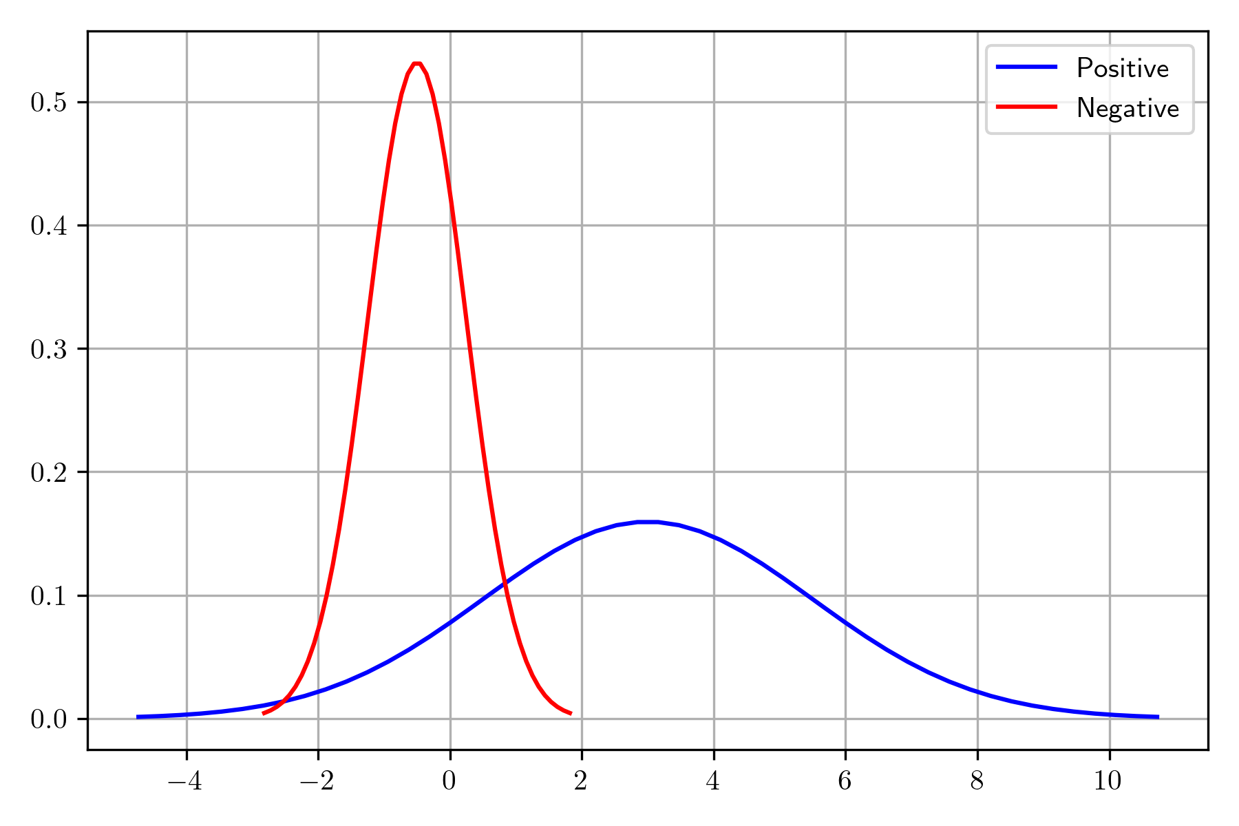
In order to illustrate the process of computing the posterior, the following example uses two normals, each one corresponding to a different class; the red one is the negative class, and blue is used to depict the positive one.
pos = norm(loc=3, scale=2.5)
neg = norm(loc=-0.5, scale=0.75)
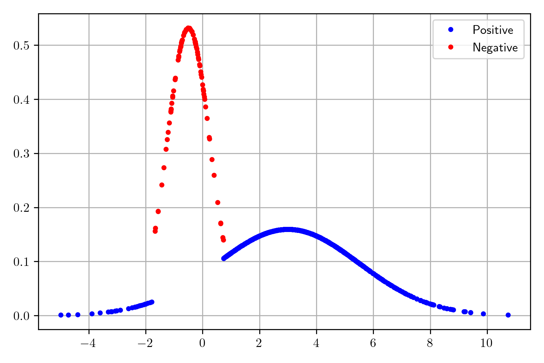
The normal associated with the negative class is sampled 100 times; however, the sampled elements in the tail corresponding to a mass lower than 0.05 or higher than 0.95 are discarded. The distribution of the positive class is sampled 1000 times using the constraint that the points in the interval of the negative class are not considered.
_min = neg.ppf(0.05)
_max = neg.ppf(0.95)
D = [(x, 0) for x in neg.rvs(100) if x >= _min and x <= _max]
D += [(x, 1) for x in pos.rvs(1000) if x < _min or x > _max]
The following picture shows the distribution of the positive and negative classes; it can be observed that the two classes are separated by the constraints imposed. These points will be used to illustrate the procedure to estimate the posterior distribution given a dataset; the dataset is \(\mathcal D=\{(x_i, y_i) \mid i=1, \ldots, N\}\) where \(x_i \in \mathbb R\) and \(y_i \in \{0, 1\}\).
The first step is to estimate the likelihood, i.e., \(\mathbb P(\mathcal X \mid \mathcal Y)\) where \(\mathcal Y=1\) and \(\mathcal Y=0\). It is assumed that the likelihood is normally distributed; thus, it requires estimating the mean and the standard deviation, which can be done with the following code.
l_pos = norm(*norm.fit([x for x, k in D if k == 1]))
l_neg = norm(*norm.fit([x for x, k in D if k == 0]))
The second step is to compute the prior, i.e., \(\mathbb P(\mathcal Y)\) which corresponds to estimating the parameters of a Categorical distribution; the following code relies on the use of np.unique to estimate them.
_, priors = np.unique([k for _, k in D], return_counts=True)
N = priors.sum()
prior_pos = priors[1] / N
prior_neg = priors[0] / N
The next step requires computing the unnormalized posterior \(\mathbb P(\mathcal X \mid \mathcal Y) \mathbb P(\mathcal Y)\); in the following example, this term is computed for all the inputs in \(\mathcal D\). The first line retrieves the inputs, i.e., \(x\). The second and third lines compute \(\mathbb P(\mathcal X \mid \mathcal Y) \mathbb P(\mathcal Y)\) for the positive and negative class.
x = np.array([x for x, _ in D])
post_pos = l_pos.pdf(x) * prior_pos
post_neg = l_neg.pdf(x) * prior_neg
The final steps are to calculate the evidence, \(\mathbb P(\mathcal X)\) and use it to normalize \(\mathbb P(\mathcal X \mid \mathcal Y) \mathbb P(\mathcal Y)\). The first line computes the evidence, and the second and four lines normalize the posterior.
evidence = post_pos + post_neg
post_pos /= evidence
post_neg /= evidence
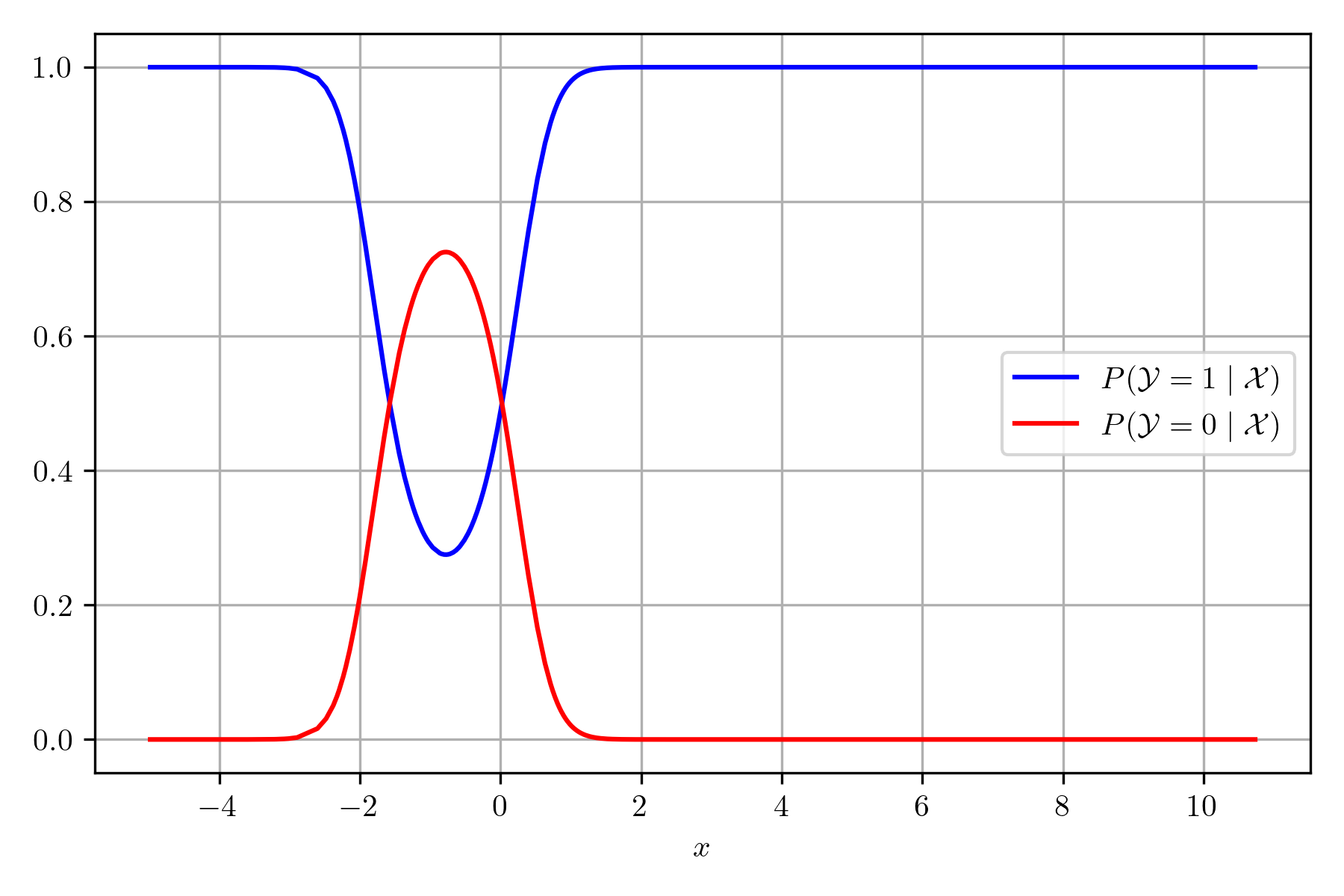
The following figure presents the posterior for each class; it can be observed that the most probable class swaps from positive to negative in the cross of the two lines.
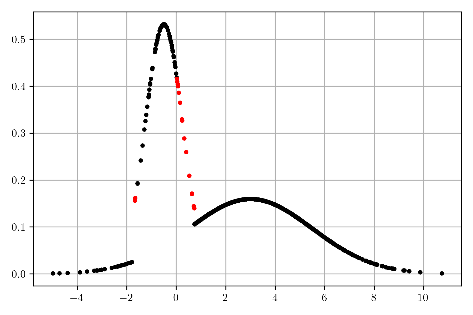
Once the posterior is estimated, it can be used to predict the class of \(x\); given that the truth class of any \(x\) in \(\mathcal D\) is known, it is possible to know when the classifier makes a mistake. The following figure depicts the data in \(\mathcal D\), marking in red those points where the classifier and truth class differs. The function to predict the class can be implemented with the following code; it is worth mentioning that it is not needed to normalize the posterior because the interest is only on the class.
klass = lambda x: 1 if l_pos.pdf(x) * prior_pos > l_neg.pdf(x) * prior_neg else 0
Multivariate Normal Distribution
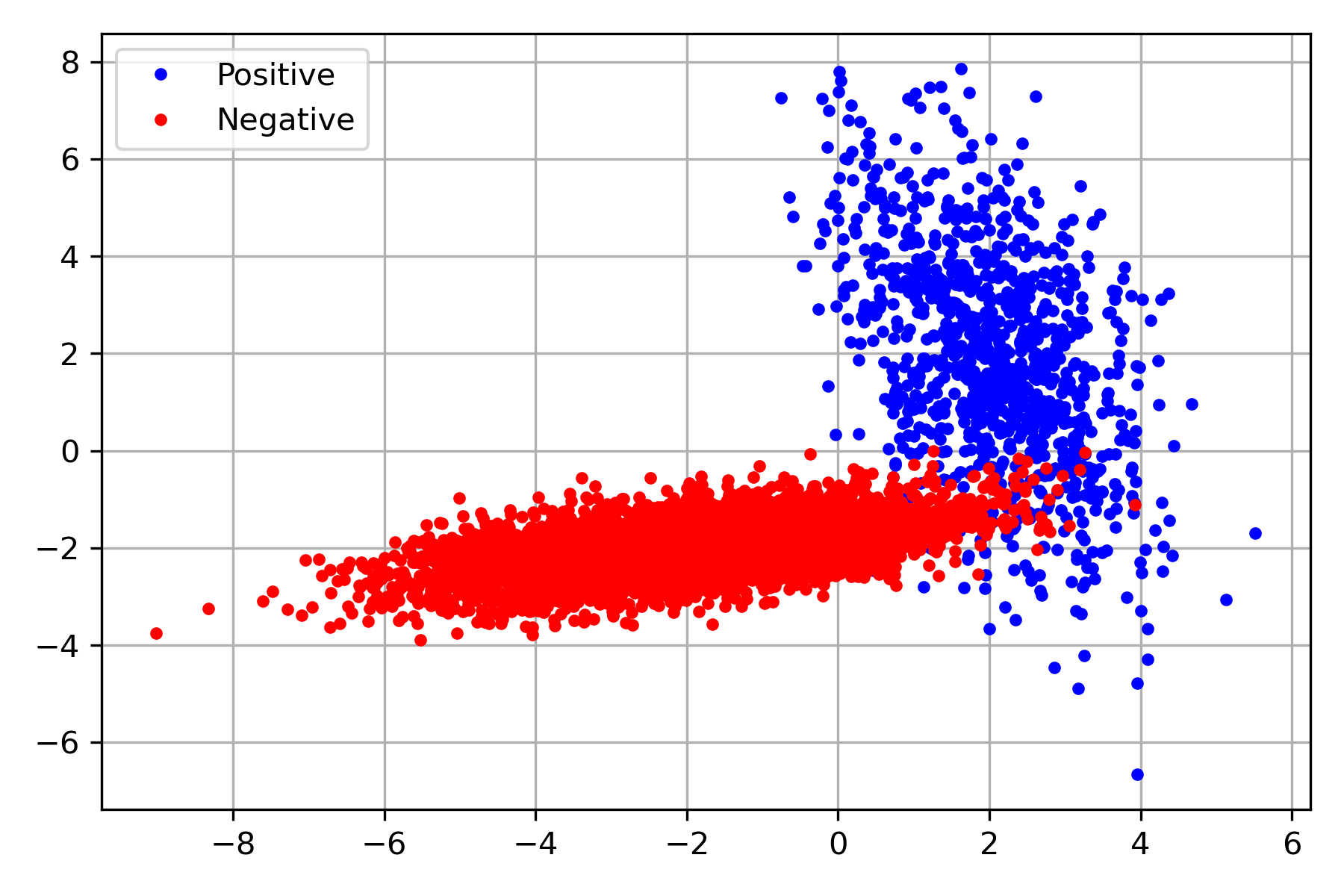
An equivalent procedure can be done for multivariate Normal distribution. The following figure shows an example of two multivariate distributions; one represents a positive class (blue), and the other corresponds to the negative (red). The dataset containing the pairs, \((\mathbf x, y)\), is found on the variable D.
D = load_model(join('dataset', 'two_classes_multivariate.gz'))
Dataset \(\mathcal D\) can be used to estimate the posterior distribution, where the first step is to estimate the parameters of the likelihood, one set of parameters for each class. The second step is to calculate the parameters of the prior. The sum of the product of these two components corresponds to the evidence, which provides all elements to compute the posterior distribution.
The following code computes the likelihood for the positive and negative class.
l_pos_m = np.mean(np.array([x for x, y in D if y == 1]), axis=0)
l_pos_cov = np.cov(np.array([x for x, y in D if y == 1]).T)
l_pos = multivariate_normal(mean=l_pos_m, cov=l_pos_cov)
l_neg_m = np.mean(np.array([x for x, y in D if y == 0]), axis=0)
l_neg_cov = np.cov(np.array([x for x, y in D if y == 0]).T)
l_neg = multivariate_normal(mean=l_neg_m, cov=l_neg_cov)
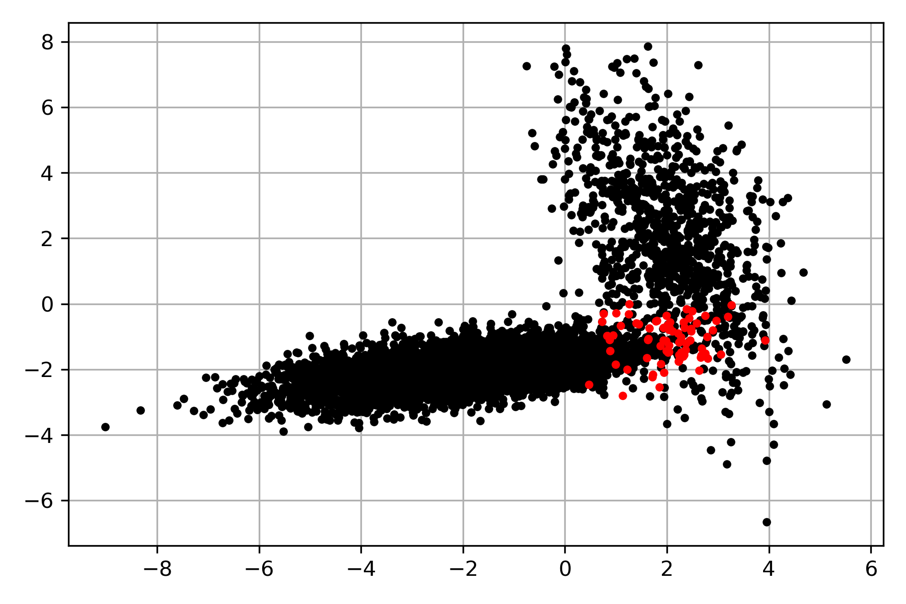
Once the likelihood has been estimated, it is straightforward to estimate the prior and the evidence and, with that, be able to compute the posterior probability. The posterior distribution can be used to predict the class for each point in \(\mathcal D\). The following figure shows in red the points in \(\mathcal D\) where the truth class is different from the predicted posterior distribution.
Categorical Distribution
The description of Bayes’ theorem continues with an example of a Categorical distribution. A Categorical distribution can simulate the drawn of \(K\) events that can be encoded as characters, and \(\ell\) repetitions can be represented as a sequence of characters. Consequently, the distribution can illustrate the generation sequences associated with different classes, e.g., positive or negative.
The first step is to create the dataset. As done previously, two distributions are defined, one for each class; it can be observed that each distribution has different parameters. The second step is to sample these distributions; the distributions are sampled 1000 times with the following procedure. Each time, a random variable representing the number of outcomes taken from each distribution is drawn from a Normal \(\mathcal N(15, 3)\) and stored in the variable length. The random variable indicates the number of outcomes for each Categorical distribution; the results are transformed into a sequence, associated to the label corresponding to the positive and negative class, and stored in the list D.
pos = multinomial(1, [0.20, 0.20, 0.35, 0.25])
neg = multinomial(1, [0.35, 0.20, 0.25, 0.20])
length = norm(loc=15, scale=3)
D = []
m = {k: chr(122 - k) for k in range(4)}
id2w = lambda x: " ".join([m[_] for _ in x.argmax(axis=1)])
for l in length.rvs(size=1000):
    D.append((id2w(pos.rvs(round(l))), 1))
    D.append((id2w(neg.rvs(round(l))), 0))
The following table shows four examples of this process; the first column contains the sequence, and the second the associated label.
| Text | Label |
|---|---|
| x w x x z w y | positive |
| y w z z z x w | negative |
| z x x x z x z w x w | positive |
| x w z w y z z z z w | negative |
As done previously, the first step is to compute the likelihood given that dataset; considering that the data comes from a Categorical distribution, the procedure to estimate the parameters is similar to the ones used to estimate the prior. The following code estimates the data parameters corresponding to the positive class. It can be observed that the parameters estimated are similar to the ones used to generate the dataset.
D_pos = []
[D_pos.extend(data.split()) for data, k in D if k == 1]
words, l_pos = np.unique(D_pos, return_counts=True)
w2id = {v: k for k, v in enumerate(words)}
l_pos = l_pos / l_pos.sum()
l_pos
array([0.25489421, 0.33854064, 0.20773186, 0.1988333 ])
An equivalent procedure is performed to calculate the likelihood of the negative class.
D_neg = []
[D_neg.extend(data.split()) for data, k in D if k == 0]
_, l_neg = np.unique(D_neg, return_counts=True)
l_neg = l_neg / l_neg.sum()
The prior is estimated with the following code, equivalent to the one used on all the examples seen so far.
_, priors = np.unique([k for _, k in D], return_counts=True)
N = priors.sum()
prior_pos = priors[1] / N
prior_neg = priors[0] / N
Once the parameters have been identified, these can be used to predict the class of a given sequence. The first step is to compute the likelihood, e.g., \(\mathbb P(\)w w x z\(\mid \mathcal Y)\). It can be observed that the sequence needs to be transformed into tokens which can be done with the split method. Then, the token is converted into an index using the mapping w2id; once the index is retrieved, it can be used to obtain the parameter associated with the word. The likelihood is the product of all the probabilities; however, this product is computed in log space.
def likelihood(params, txt):
    params = np.log(params)
    _ = [params[w2id[x]] for x in txt.split()]
    tot = sum(_)
    return np.exp(tot)
The likelihood combined with the prior for all the classes produces the evidence, which subsequently is used to calculate the posterior distribution. The posterior is then used to predict the class for all the sequences in \(\mathcal D\). The predictions are stored in the variable hy.
post_pos = [likelihood(l_pos, x) * prior_pos for x, _ in D]
post_neg = [likelihood(l_neg, x) * prior_neg for x, _ in D]
evidence = np.vstack([post_pos, post_neg]).sum(axis=0)
post_pos /= evidence
post_neg /= evidence
hy = np.where(post_pos > post_neg, 1, 0)
Accuracy
In previous examples, figures have been used to depict the classification errors; however, it is not practical to rely on a figure to evaluate the classifier’s performance. Instead, one can use a performance measure to assess the classifier’s quality. The first performance measure revised is the accuracy. The accuracy is the ratio of correct predictions.
The accuracy of the classifier trained previously is computed with the following code, where variable hy contains the predictions and y contains the classes taken from \(\mathcal D\).
y = np.array([y for _, y in D])
(hy == y).mean()
0.761
Confidence Interval
Like any other performance measure applied in this domain, the accuracy can change when the experiment is repeated; sampling the distributions and creating a new dataset would produce a different accuracy. Therefore, to have a complete picture of the classifier’s performance, it is needed to estimate the difference values this measure can have under the same circumstances. One approach is to calculate the confidence interval of the performance measure used. A standard method to compute the confidence interval assumes that it is normally distributed when the size of \(\mathcal D\) tends to infinity; in this condition, the confidence interval is \((\hat \theta - z_{\frac{\alpha}{2}}\hat{\textsf{se}}, \hat \theta + z_{\frac{\alpha}{2}}\hat{\textsf{se})}\), where \(\hat \theta\) is the point estimation, e.g., the accuracy, \(z_{\frac{\alpha}{2}}\) is the point where the mass is \(1-\frac{\alpha}{2}\), and \(\hat{\textsf{se}} = \sqrt{\mathbb V(\hat \theta)}\) is the standard error.
The accuracy is the sum of \(N\) Bernoulli trials, therefore \(\sqrt{\mathbb V(\hat \theta)}\) is \(\sqrt{\frac{p(1-p)}{N}}\) where \(p\) is the accuracy. Using these elements the confidence interval for the accuracy is computed as follows.
p = (hy == y).mean()
se = np.sqrt(p * (1 - p) / y.shape[0])
coef = norm.ppf(0.975)
ci = (p - coef * se, p + coef * se)
ci
(0.7423093514177674, 0.7796906485822326)
The standard error of the accuracy can be derived using the identity \(\mathbb V(\sum_i a_i \mathcal X_i) = \sum_i a_i^2 \mathbb V(\mathcal X_i)\) where random variables \(\mathcal X_i\) are independent and \(a_i\) is a constant. On the other hand, the accuracy can be seen as the outcome of a random variable where \(1\) indicates the correct prediction and \(0\) represents an error, then the accuracy is the sum of these random variables. Let \(\mathcal X_i\) represent the outcome of the \(i\)-th prediction, then the accuracy is \(\frac{1}{N} \sum_i^N X_i\). The variance is \(\mathbb V(\frac{1}{N} \sum_i^N X_i) = \sum_i \frac{1}{N^2} \mathbb V(\mathcal X_i)\); the variance of a Bernoulli distribution with parameter \(p\) is \(p(1-p)\), consequently \(\sum_i \frac{1}{N^2} \mathbb V(\mathcal X_i) = \frac{1}{N^2} \sum_i p(1-p) = \frac{1}{N}p(1-p)\), which completes the derivation.
There are performance measures that it is difficult or unfeasible to analytical obtain \(\sqrt{\mathbb V(\hat \theta)}\), for those cases, one can use a bootstrapping method to estimate it, the following code shows the usage of a method that implements the bootstrap percentile interval when the performance measure is the accuracy. However, it can be observed that the measure is a parameter of the method, so it works for any performance measure.
ci = bootstrap_confidence_interval(y, hy, alpha=0.05,
                                  metric=lambda a, b: (a == b).mean())
ci
(0.7415, 0.7797625)
Text Categorization - Categorical Distribution
The approach followed on text categorization is to treat it as supervised learning problem where the starting point is a dataset \(\mathcal D = \{(\text{text}_i, y_i) \mid i=1,\ldots, N\}\) where \(y \in \{c_1, \ldots c_K\}\) and \(\text{text}_i\) is a text. For example, the next code uses a toy sentiment analysis dataset with four classes: negative (N), neutral (NEU), absence of polarity (NONE), and positive (P).
D = [(x['text'], x['klass']) for x in tweet_iterator(TWEETS)]
As can be observed, \(\mathcal D\) is equivalent to the one used in the Categorical Distribution example. The difference is that sequence of letters is changed with a sentence. Nonetheless, a feasible approach is to obtain the tokens using the split method. Another approach is to retrieve the tokens using a Tokenizer, as covered in the Text Normalization Section.
The following code uses the TextModel class to tokenize the text using words as the tokenizer; the tokenized text is stored in the variable D.
tm = TextModel(token_list=[-1])
tok = tm.tokenize
D = [(tok(x), y) for x, y in D]
Before estimating the likelihood parameters, it is needed to encode the tokens using an index; by doing it, it is possible to store the parameters in an array and compute everything numpy operations. The following code encodes each token with a unique index; the mapping is in the dictionary w2id.
words = set()
[words.update(x) for x, y in D]
w2id = {v: k for k, v in enumerate(words)}
Previously, the classes have been represented using natural numbers. The positive class has been associated with the number \(1\), whereas the negative class with \(0\). However, in this dataset, the classes are strings. It was decided to encode them as numbers to facilitate subsequent operations. The encoding process can be performed simultaneously with the estimation of the prior of each class. Please note that the priors are stored using the logarithm in the variable priors.
uniq_labels, priors = np.unique([k for _, k in D], return_counts=True)
priors = np.log(priors / priors.sum())
uniq_labels = {str(v): k for k, v in enumerate(uniq_labels)}
It is time to estimate the likelihood parameters for each of the classes. It is assumed that the data comes from a Categorical distribution and that each token is independent. The likelihood parameters can be stored in a matrix (variable l_tokens) with \(K\) rows, each row contains the parameters of the class, and the number of columns corresponds to the vocabulary’s size. The first step is to calculate the frequency of each token per class which can be done with the following code.
l_tokens = np.zeros((len(uniq_labels), len(w2id)))
for x, y in D:
    w = l_tokens[uniq_labels[y]]
    cnt = Counter(x)
    for i, v in cnt.items():
        w[w2id[i]] += v
The next step is to normalize the frequency. However, before normalizing it, it is being used a Laplace smoothing with a value \(0.1\). Therefore, the constant \(0.1\) is added to all the matrix elements. The next step is to normalize (second line), and finally, the parameters are stored using the logarithm.
l_tokens += 0.1
l_tokens = l_tokens / np.atleast_2d(l_tokens.sum(axis=1)).T
l_tokens = np.log(l_tokens)
Prediction
Once all the parameters have been estimated, it is time to use the model to classify any text. The following function computes the posterior distribution. The first step is to tokenize the text (second line) and compute the frequency of each token in the text. The frequency stored in the dictionary cnt is converted into the vector x using the mapping function w2id. The final step is to compute the product of the likelihood and the prior. The product is computed in log-space; thus, this is done using the likelihood and the prior sum. The last step is to compute the evidence and normalize the result; the evidence is computed with the function logsumexp.
def posterior(txt):
    x = np.zeros(len(w2id))
    cnt = Counter(tm.tokenize(txt))
    for i, v in cnt.items():
        try:
            x[w2id[i]] += v
        except KeyError:
            continue
    _ = (x * l_tokens).sum(axis=1) + priors
    l = np.exp(_ - logsumexp(_))
    return l
The posterior function can predict all the text in \(\mathcal D\); the predictions are used to compute the model’s accuracy. In order to compute the accuracy, the classes in \(\mathcal D\) need to be transformed using the nomenclature of the likelihood matrix and priors vector; this is done with the uniq_labels dictionary (second line).
hy = np.array([posterior(x).argmax() for x, _ in D])
y = np.array([uniq_labels[y] for _, y in D])
(y == hy).mean()
0.974
Training
Solving supervised learning problems requires two phases; one is the training phase, and the other is the prediction. The posterior function handles the later phase, and it is missing to organize the code described in a training function. The following code describes the training function; it requires the dataset’s parameters and an instance of TextModel.
def training(D, tm):
    tok = tm.tokenize
    D =[(tok(x), y) for x, y in D]
    words = set()
    [words.update(x) for x, y in D]
    w2id = {v: k for k, v in enumerate(words)}
    uniq_labels, priors = np.unique([k for _, k in D], return_counts=True)
    priors = np.log(priors / priors.sum())
    uniq_labels = {str(v): k for k, v in enumerate(uniq_labels)}
    l_tokens = np.zeros((len(uniq_labels), len(w2id)))
    for x, y in D:
        w = l_tokens[uniq_labels[y]]
        cnt = Counter(x)
        for i, v in cnt.items():
            w[w2id[i]] += v
    l_tokens += 0.1
    l_tokens = l_tokens / np.atleast_2d(l_tokens.sum(axis=1)).T
    l_tokens = np.log(l_tokens)
    return w2id, uniq_labels, l_tokens, priors
Performance
The performance of a supervised learning algorithm cannot be measured on the same data where it was trained. To illustrate this issue, imagine an algorithm that memorizes the dataset, and for all inputs that have not been seen, the algorithm outputs a random class. Consequently, this algorithm is useless because it cannot be used to predict an input outside the dataset used to train it. Nonetheless, it has a perfect score, in any performance measure, in the dataset used to estimate its parameters.
Traditionally, this issue is handle by splitting the dataset \(\mathcal D\) into two disjoint sets, \(\mathcal D = \mathcal T \cup \mathcal G\) where \(\mathcal T \cap \mathcal G = \emptyset\), or three sets \(\mathcal D = \mathcal T \cup \mathcal V \cup \mathcal G\) where \(\mathcal T \cap \mathcal V \cap \mathcal G = \emptyset\). The set \(\mathcal T\), known as training set, is used to train the algorithm, i.e., to estimate the parameters, whereas the set \(\mathcal G\), known as test set or gold set, is used to measure its performance. The set \(\mathcal V\), known as validation set, is used to optimize the algorithm’s hyperparameters; for example, a hyperparameter in an n-gram language model is the value of \(n\).
KFold and StratifiedKFold
There are scenarios where the size of \(\mathcal D\) prohibits splitting it in training, validation and test sets; for this case, an alternative approach is to split \(\mathcal D\) several times with a different selection each time. The process is known as k-fold cross-validation when all the elements in \(\mathcal D\) are used once in a validation set. For example, the k-fold cross-validation when \(k=3\) corresponds to the following process. The set \(\mathcal D\) is split into three disjoint sets \(\mathcal D_1, \mathcal D_2, \mathcal D_3\) where \(\mathcal D=\mathcal D_1 \cup \mathcal D_2 \cup \mathcal D_3;\) with the characteristic that all the subsets have a similar cardinality. These datasets are used to create three training and validation sets, i.e., \(\mathcal T_1=\mathcal D_2 \cup \mathcal D_3\), \(\mathcal V_1=\mathcal D_1\), \(\mathcal T_2=\mathcal D_1 \cup \mathcal D_3\), \(\mathcal V_2=\mathcal D_2\), and \(\mathcal T_3=\mathcal D_1 \cup \mathcal D_2\), \(\mathcal V_3=\mathcal D_3.\) As can be observed all the elements in \(\mathcal D\) are used once in a validation set.
The only constraints imposed in a k-fold cross are that all validation sets have a similar cardinality and that all the elements in \(\mathcal D\) appear once. For problems where the proportion of the different classes is unbalanced, adding another constraint in the selection process is helpful; the constraint is to force the distribution of classes to remain similar in all the validation sets. This latter process is known as stratified k-fold cross-validation.
The following code implements stratified k-fold cross-validation, predicts all the elements in \(\mathcal D\), and stores the predictions in the variable hy.
D = [(x['text'], x['klass']) for x in tweet_iterator(TWEETS)]
tm = TextModel(token_list=[-1])
folds = StratifiedKFold(shuffle=True, random_state=0)
hy = np.empty(len(D))
for tr, val in folds.split(D, y):
    _ = [D[x] for x in tr]
    w2id, uniq_labels, l_tokens, priors = training(_, tm)
    hy[val] = [posterior(D[x][0]).argmax() for x in val]
Once the classes in \(\mathcal D\) has been predicted, one can compute the accuracy of the classifier with the following code. It can be observed that the accuracy is lower than the one obtained when it was measured on the same data used to estimate the parameters.
y = np.array([uniq_labels[y] for _, y in D])
(y == hy).mean()
0.618
The confidence interval of the accuracy is computed as follows.
p = (hy == y).mean()
s = np.sqrt(p * (1 - p) / y.shape[0])
coef = norm.ppf(0.975)
ci = (p - coef * s, p + coef * s)
ci
(0.5878856141926456, 0.6481143858073544)
Precision, Recall, and F1-score
The accuracy is a popular performance measure; however, it has drawbacks. For example, in a dataset where one class is more frequent than the other, e.g., there are 99 examples of the negative class and only one example of the positive one, then the accuracy for the classifier that always predicts negative is .99. This performance can be seen as adequate; however, the classifier defined is constant, not even looking at the inputs.
Other famous metrics used in classification are precision, recall, and score \(f_1\). These performance measures are defined on binary classification problems; however, k-class classification problems can be codified as \(k\) binary problems; in each of these problems, the positive class is one of the classes, and the negative class is the union of the rest of the classes.
The precision is the proportion of correct classification of positive objects, that is, \(\textsf{precision}(\mathbf y, \hat{\mathbf y}) = \frac{\sum_i \mathbb 1(\mathbf y_i = 1) \mathbb 1(\mathbf{\hat y_i} = 1) }{\sum_i \mathbb 1(\mathbf{ \hat y_i = 1})}.\) On the other hand, the recall is \(\textsf{recall}(\mathbf y, \hat{\mathbf y}) = \frac{\sum_i \mathbb 1(\mathbf y_i = 1) \mathbb 1(\mathbf{\hat y_i} = 1) }{\sum_i \mathbb 1(\mathbf{y_i = 1})}.\) The next code uses two functions from sklearn to compute the precision and recall.
p = precision_score(y, hy, average=None)
r = recall_score(y, hy, average=None)
Furthermore, the score \(f_1\) is defined in terms of the precision and recall; it is the harmonic mean \(f_1 = 2 \frac{\textsf{precision} \cdot \textsf{recall}}{\textsf{precision} + \textsf{recall}}\).
f1_score(y, hy, average=None)
The precision, recall, and score \(f_1\) are defined on binary classification problems, and these measures are most of the time computed for the positive class; however, nothing prohibits computing it for the other class; in the previous code, it is only needed to change \(1\) to \(0\). Additionally, it is possible to calculate these measures for all the classes in a \(K\) classification problem, and the result is to have one measure per class; the average of these values is known as macro. The following code computes the confidence interval of the macro-recall obtained from the predictions of \(\mathcal D\) using stratified k-fold cross-validation.
metric = lambda a, b: recall_score(a, b, average='macro')
ci = bootstrap_confidence_interval(y, hy,
                                   metric=metric)
ci
(0.4006296585578326, 0.4415247767402683)
Tokenizer
One of the critical components in the text categorization algorithm is the method used to tokenize the text; changing the tokenizer’s parameters impacts the classifier’s performance, e.g., the following code shows an example where the tokenizer used the default parameters. An increase in performance can be observed, albeit both confidence intervals overlap, so it cannot be concluded that one set of parameters is better than the other.
tm = TextModel()
hy = np.empty(len(D))
for tr, val in folds.split(D, y):
    T = [D[x] for x in tr]
    w2id, uniq_labels, l_tokens, priors = training(T, tm)
    assert np.all(np.isfinite([posterior(D[x][0]) for x in val]))
    hy[val] = [posterior(D[x][0]).argmax() for x in val]

y = np.array([uniq_labels[y] for _, y in D])
metric = lambda a, b: recall_score(a, b, average='macro')
ci = bootstrap_confidence_interval(y, hy,
                                   metric=metric)
ci
(0.4326075670113598, 0.47454989683417365)