Collocations
Contents
- Introduction
- Bernoulli Distribution
- Categorical distribution
- Bivariate distribution
- Hypothesis Testing
- Activities
Libraries used
from text_models import Vocabulary
from collections import Counter
import numpy as np
from scipy.stats import norm, chi2
from wordcloud import WordCloud as WC
from matplotlib import pylab as plt
Installing external libraries
pip install microtc
pip install evomsa
pip install text_models
Introduction
A collocation is an expression with the characteristic that its meaning cannot be inferred by simply adding the definition of each of its words, e.g., kick the bucket.
As can be expected, finding a collocation is a challenging task; one needs to know the meaning of the words and then realize that the combination of these words produces an utterance that its components cannot explain. However, the approach taken here is more limited; instead of looking for a sentence of any length, we will analyze bigrams and describe algorithms that can retrieve bigrams that could be considered collocations.
The frequency of the bigrams can be represented in a co-occurrence matrix as the one shown in the following table.
| the | to | of | in | and | |
|---|---|---|---|---|---|
| the | 0 | 33390 | 23976 | 29159 | 22768 |
| to | 33390 | 0 | 10145 | 18345 | 17816 |
| of | 23976 | 10145 | 0 | 6683 | 7802 |
| in | 29159 | 18345 | 6683 | 0 | 11536 |
| and | 22768 | 17816 | 7802 | 11536 | 0 |
The co-occurrence matrix was created using the data obtained from the library text_models (see A Python library for exploratory data analysis on twitter data based on tokens and aggregated origin–destination information) using the following code. The third line retrieves all the bigrams and stores them in the variable bigrams. The loop goes for all the bigrams that contains one of the five words defined in index, it is observed that the matrix is symmetric, this is because the text_models library does not store the order of the words composing the bigram.
date = dict(year=2022, month=1, day=10)
voc = Vocabulary(date, lang='En', country="US")
bigrams = Counter({k: v for k, v in voc.voc.items() if k.count("~")})
co_occurrence = np.zeros((5, 5))
index = {'the': 0, 'to': 1, 'of': 2, 'in': 3, 'and': 4}

for bigram, cnt in bigrams.most_common():
    a, b = bigram.split('~')
    if a in index and b in index:
        co_occurrence[index[a], index[b]] = cnt
        co_occurrence[index[b], index[a]] = cnt
The idea is to use the information of the co-occurrence matrix to find the pairs of words that can be considered collocations. The first step is to transform the co-occurrence matrix into a bivariate distribution and then use statistical approaches to retrieve some prominent pairs. Before going into the details of these algorithms, it is pertinent to describe the relationship between words and random variables.
Each element in the matrix can be uniquely identified by the pair words, e.g., the frequency of pair (in, of) is \(6683\). However, it is also possible to identify the same element using an index. For example, if the first word (the) is assigned the index \(0\), the index \(3\) corresponds to word in and \(2\) to of. Consequently, the element (in, of) can uniquely identify with the pair (3, 2). One can create a mapping between words and natural numbers such that each different word has a unique identifier. The mapping allows working with natural numbers instead of words which facilitates the analysis and returns to the words (using the inverse mapping) when the result is obtained.
The mapping can be implemented using a dictionary, as seen from the following code where the variable of interest is index.
for bigram, cnt in bigrams.items():
    a, b = bigram.split('~')
    for x in [a, b]:
        if x not in index:
            index[x] = len(index)
len(index)
41419
It is essential to mention that a random variable is a mapping that assigns a real number to each outcome. In this case, the outcome is observing a word and the mapping is the transformation of the word into the natural number.
The co-occurrence matrix contains the information of two random variables; each one can have \(d\) (length of the dictionary) different outcomes. Sometimes, working with two random variables might be challenging, so a more suitable approach is starting the description with the most simple case, which corresponds to a single random variable with only two outcomes.
Bernoulli Distribution
Let \(\mathcal{X}\) be a random variable with two outcomes (\(\{1, 0\}\)), e.g., this variable corresponds to a language that only has two words. At this point, one might realize that different experiments can be represented with a random variable of two outcomes; perhaps the most famous one is tossing a coin.
The random variable \(\mathcal{X}\) has a Bernoulli distribution, i.e., \(\mathcal X \sim \textsf{Bernoulli}(p)\), in the case that \(\mathbb P(\mathcal X=1)=p\) and \(\mathbb P(\mathcal X=0)=1 - p\) for \(p \in [0, 1]\), where the probability (mass) function is \(f_{\mathcal X}(x) = p^x(1-p)^{1-x}.\)
For example, the language under study has two words good and bad, and we encountered a sequence “good bad bad good good.” Using the following mapping
\[\mathcal X(w) = \begin{cases} 1 \text{ when } w \text{ is good}\\ 0 \text{ when } w \text{ is bad} \end{cases}.\]The sequence is represented as \((1, 0, 0, 1, 1)\) and in general a sequence of five elements is \((\mathcal X_1, \mathcal X_2, \mathcal X_3, \mathcal X_4, \mathcal X_5);\) as expected a sequence of \(N\) observations is \((\mathcal X_1, \mathcal X_2, \ldots, \mathcal X_N)\). Different studies can be applied to a sequence; however, at this point we would like to impose some constraints on the way it was obtained. The first constraint is to assume that \(\mathcal X_i \sim \textsf{Bernoulli}(p),\) then one is interested in estimating the value of the parameter \(p\). The second assumption is that the random variables are indepedent, that is, the outcome of the variable \(\mathcal X_i\) is independent of \(\mathcal X_j\) for \(j \neq i.\)
There is an important characteristic for independent random variables, i.e., \((\mathcal X_1, \mathcal X_2, \ldots, \mathcal X_N)\) which is
\[\mathbb P(\mathcal X_1, \mathcal X_2, \ldots, \mathcal X_N) = \prod_{i=1}^N \mathbb P(\mathcal X_i).\]Returning to the example “good bad bad good good,” the independent assumption means that observing bad as the second word is not influenced by getting good as the first word.
Maximum Likelihood Method
A natural example of independent random variables is the tossing of a coin. For example, observing the sequence \((1, 0, 0, 1, 1)\) and knowing that these come from tossing a coin five times, then our intuition indicates that the estimated parameter \(p\) correspond to the fraction between the number of ones (3) and the number of tosses (5).
A natural example of independent random variables is the tossing of a coin. For example, observing the sequence \((1, 0, 0, 1, 1)\) and knowing that these come from tossing a coin five times, then our intuition indicates that the estimated parameter \(p\) correspond to the fraction between the number of ones (3) and the number of tosses (5). In this case, our intuition corresponds to the maximum likelihood method defined as follows:
\[\mathcal L_{f_{\mathcal X}}(\theta) = \prod_{i=1}^N f_{\mathcal X}(x_i \mid \theta),\]where \(f_{\mathcal X}\) corresponds to the probability density function, in the case discrete random variable corresponds to \(\mathbb P(X=x) = f_{\mathcal X}(x),\) and the notation \(f_{\mathcal X}(x_i \mid \theta)\) indicates that \(f\) depends on a set of parameters refered as \(\theta\).
The maximum likelihood estimator \(\hat \theta\) corresponds to maximizing \(\mathcal L_{f_{\mathcal X}}(\theta)\) or equivalent maximizing \(l_{f_\mathcal X}(\theta) = \log \mathcal L_{f_{\mathcal X}}(\theta).\)
Continuing with the example \((1, 0, 0, 1, 1)\), given that \(\mathcal X_i\) is Bernoulli distributed then \(f_{\mathcal X}(x) = p^x(1-p)^{1-x}\). The maximum likelihood estimator of \(p\) is obtained by maximizing the likelihood function, which can be solved analytically by following the next steps.
\[\begin{eqnarray} \frac{d}{dp} \mathcal l_{f_{\mathcal X}}(p) &=& 0 \\ \frac{d}{dp} [ \sum_{i=1}^N x_i \log p + (1-x_i) \log (1 - p)] &=& 0 \\ \frac{d}{d p} [ \sum_{i=1}^N x_i \log p + \log (1 - p) (N - \sum_{i=1}^N x_i) ] &=& 0\\ \sum_{i=1}^N x_i \frac{d}{d p} \log \mathcal p + (N - \sum_{i=1}^N x_i) \frac{d}{d p} \log (1 - \mathcal p) &=& 0\\ \sum_{i=1}^N x_i \frac{1}{p} + (N - \sum_{i=1}^N x_i) \frac{-1}{(1 - p)} &=& 0 \\ \end{eqnarray},\]solving for \(p\) it is obtained \(\hat p = \frac{1}{N}\sum_{i=1}^N x_i.\)
For example, the following code creates an array of 100 elements where each element is the outcome of a Bernoulli distributed random variable. The second line estimates the parameter \(p\).
x = np.random.binomial(1, 0.3, size=100)
hp = x.mean()
Categorical distribution
Having a language with only two words seems useless; it sounds more realistic to have a language with \(d\) words. Let \(\mathcal X\) be a random variable with \(d\) outcomes (\(\{1, 2, \ldots, d\}\)). The random variable \(\mathcal X\) has a Categorical distribution, i.e., \(\mathcal X \sim \textsf{Categorical}(\mathbf p)\) in the case \(\mathbb P(\mathcal X=i) = \mathbf p_i\) for \(1 \leq i \leq d\), where \(\sum_i^d \mathbf p_i =1\) and \(\mathbf p \in \mathbb R^d\). The probability mass function of a Categorical distribution is \(f_{\mathcal X}(x) = \prod_{i=1}^d \mathbf p_i^{\mathbb 1(i=x)}\).
The estimated parameter is \(\hat{\mathbf p}_i = \frac{1}{N}\sum_{j=1}^N \mathbb 1(x_j = i).\)
Maximum Likelihood Estimator
The maximum likelihood estimator can be obtained by maximizing the log-likelihood, i.e.,
\[l_{f_\mathcal X}(\mathbf p) = \log \prod_{i=1}^N \prod_{k=1}^d \mathbf p_k^{\mathbb 1(x_i=k)},\]subject to the constraint \(\sum_i^d \mathbf p_i=1\).
An optimization problem with a equality constraint can be solved using Langrage multipliers which requieres setting the constraint in the original formulation and making a derivative on a introduce variable \(\lambda\). Using Langrage multiplier the system of equations that need to be solved is the following:
\[\begin{eqnarray} \frac{\partial}{\partial \mathbf p_j} [\log \prod_{i=1}^N \prod_{k=1}^d \mathbf p_k^{\mathbb 1(x_i=k)} - \lambda (\sum_i^d \mathbf p_i -1)] &=& 0 \\ \frac{\partial}{\partial \lambda} [\log \prod_{i=1}^N \prod_{k=1}^d \mathbf p_k^{\mathbb 1(x_i=k)} - \lambda (\sum_i^d \mathbf p_i -1)] &=& 0 \\ \end{eqnarray},\]where the term \(\lambda (\sum_i^d \mathbf p_i -1)\) corresponds to the equality constraint.
For example, one of the most known processes that involve a Categorical distribution is rolling a dice. The following is a procedure to simulate dice rolling using a Multinomial distribution.
X = np.random.multinomial(1, [1/6] * 6, size=100)
x = X.argmax(axis=1)
On the other hand, the maximum likelihood estimator can be implemented as follows:
var, counts = np.unique(x, return_counts=True)
N = counts.sum()
p = counts / N
Bivariate distribution
We have all the elements to realize that the co-occurrence matrix is the realization of two random variables (each one can have \(d\) outcomes); it keeps track of the number of times a bigram appear in a corpus. So far, we have not worked with two random variables; however, the good news is that the co-occurrence matrix contains all the information needed to define a bivariate distribution for this process.
The first step is to define a new random variable \(\mathcal X_i\) that represents the event of getting a bigram. \(\mathcal X_i\) is defined using \(\mathcal X_r\) and \(\mathcal X_r\) which correspond to the random variables of the first and second word of the bigram. For the case, \(\mathcal X_r=r\) and \(\mathcal X_c=c\) the random variable is defined as \(\mathcal X_i= (r + 1) \cdot (c + 1)\), where the constant one is needed in case zero is included as one of the outcomes of the random variables \(\mathcal X_r\) and \(\mathcal X_c\). For example, in the co-occurrence matrix, presented previously, the realization \(\mathcal X_r=3\) and \(\mathcal X_c=2\) corresponds to the bigram (in, of) which has a recorded frequency of \(6683\), using the new variable the event is \(\mathcal X_i=12\). As can be seen, \(X_i\) is a random variable with \(d^2\) outcomes. We can suppose \(\mathcal X_i\) is a Categorical distributed random variable, i.e., \(\mathcal X_i \sim \textsf{Categorical}(\mathbf p).\)
The fact that \(\mathcal X_i\) would be considered Categorical distributed implies that the bigrams are independent that is observing one of them is not affected by the previous words in any way. However, with this assumption it is straightforward estimating the parameter \(\mathbf p\) which is \(\hat{\mathbf p}_i = \frac{1}{N}\sum_{j=1}^N \mathbb 1(x_j = i).\). Consequently, the co-occurrence matrix can be converted into a bivariate distribution by dividing it by \(N\), where \(N\) is the sum of all the values of the co-occurrence matrix. For example, the following code builds the bivariate distribution from the co-occurrence matrix.
co_occurrence = np.zeros((len(index), len(index)))
for bigram, cnt in bigrams.most_common():
    a, b = bigram.split('~')
    if a in index and b in index:
        co_occurrence[index[a], index[b]] = cnt
        co_occurrence[index[b], index[a]] = cnt
co_occurrence = co_occurrence / co_occurrence.sum()
The following table presents an extract of the bivariate distribution.
| the | to | of | in | and | |
|---|---|---|---|---|---|
| the | 0.00000 | 0.00164 | 0.00118 | 0.00144 | 0.00112 |
| to | 0.00164 | 0.00000 | 0.00050 | 0.00090 | 0.00088 |
| of | 0.00118 | 0.00050 | 0.00000 | 0.00033 | 0.00038 |
| in | 0.00144 | 0.00090 | 0.00033 | 0.00000 | 0.00057 |
| and | 0.00112 | 0.00088 | 0.00038 | 0.00057 | 0.00000 |
Once the information of the bigrams has been transformed into a bivariate distribution, we can start analyzing it. As mentioned previously, the idea is to identify those bigrams that can be considered collocations. However, the frequency of the bigrams does not contain semantic information of the words or the phrase at hand, which can be used to identify a collocation precisely. Nonetheless, a collocation is a phrase where its components do not appear by chance; that is, the elements composing it are not drawn independently from a distribution. Therefore, the bivariate distribution can be used to identify those words that are not independent, which is a hard constraint for being considered a collocation.
Independence and Marginal Distribution
The bivariate distribution shown in the previous table contains the probability of obtaining a bigram, i.e., \(\mathbb P(\mathcal X_r=r, \mathcal X_c=c)\); this information is helpful when combined with the concept of independence and marginal distribution.
Two random variables \(\mathcal X\) and \(\mathcal Y\) are independent if \(\mathbb P(\mathcal X, \mathcal Y)=\mathbb P(\mathcal X) \mathbb P(\mathcal Y).\)
The definition of independence is useless if \(\mathbb P(\mathcal X)\) and \(\mathbb P(\mathcal Y)\) are unknown. Fortunately, the marginal distribution definition describes the procedure to obtain \(\mathbb P(\mathcal X=x)\) and \(\mathbb P(\mathcal Y=y)\) from the bivariate distribution. Let \(f_{\mathcal X, \mathcal Y}\) be the joint distribution mass function (i.e., \(f_{\mathcal X, \mathcal Y}(x, y)=\mathbb P(\mathcal X=x, \mathcal Y=y)\)) then the marginal mass function for \(\mathcal X\) is
\[f_{\mathcal X}(x) = \mathbb P(\mathcal X=x) = \sum_y \mathbb P(\mathcal X=x, \mathcal Y=y) = \sum_y f_{\mathcal X, \mathcal Y}(x, y).\]Example of rolling two dices
The interaction of these concepts can be better understood with a simple example in where all details are known. The following code simulated the rolling of two dices. Variables R and C contain the rolling of the two dices, and the variable Z has the outcome of the pair.
d = 6
R = np.random.multinomial(1, [1/d] * d, size=10000).argmax(axis=1)
C = np.random.multinomial(1, [1/d] * d, size=10000).argmax(axis=1)
Z = [[r, c] for r, c in zip(R, C)]
Z is transformed first into a frequency matrix (variable W), equivalent to a co-occurrence matrix, and then, it is converted into a bivariate distribution (last line).
W = np.zeros((d, d))
for r, c in Z:
    W[r, c] += 1
W = W / W.sum()
The next matrix presents the bivariate distribution W
The next step is to compute the marginal instributions \(\mathbb P(\mathcal X_r)\) and \(\mathbb P(\mathcal X_c)\) which can be done as follows
R_m = W.sum(axis=1)
C_m = W.sum(axis=0)
The marginal distribution and the definition of independence are used to obtain \(\mathbb P(\mathcal X_r) \mathbb P(\mathcal X_c)\) which can be computed using the dot product, consequenly R and C need to be transform into a two dimensional array using np.atleast_2d function.
ind = np.dot(np.atleast_2d(R_m).T, np.atleast_2d(C_m))
W contains the estimated bivariate distribution, and ind could be the bivariate distribution only if \(\mathcal X_r\) and \(\mathcal X_c\) are independent. The following matrix shows W-ind, which would be a zero matrix if the variables are independent.
It is observed from the matrix that all its elements are close to zero (\(\mid W_{ij}\mid \leq 0.009\)), which is expected given that by construction, the two variables are independent. On the other hand, a simulation where the variables are not independent would produce a matrix where its components are different from zero. Such an example can be quickly be done by changing variable Z. The following code simulates the case where the two dices cannot have the same value: the events \((1, 1), (2, 2), \ldots,\) are unfeasible. It is hard to imagine how this experiment can be done with two physical dice; however, simulating it is only a condition, as seen in the following code.
Z = [[r, c] for r, c in zip(R, C) if r != c]
The difference between the estimated bivariate distribution and the product of the marginal distributions is presented in the following matrix. It can be observed that the values in the diagonal are negative because \(\mathbb P(\mathcal X_r=x, \mathcal X_c=x)=0\) these events are not possible in this experiment. Additionally, the values of the diagonal are higher than \(\mid W_{ii} \mid > 0.09.\)
\[\begin{pmatrix} -0.0277 & 0.0076 & 0.0076 & 0.0026 & 0.0047 & 0.0053 \\ 0.0045 & -0.0282 & 0.0070 & 0.0058 & 0.0079 & 0.0030 \\ 0.0075 & 0.0055 & -0.0286 & 0.0051 & 0.0049 & 0.0056 \\ 0.0061 & 0.0064 & 0.0042 & -0.0272 & 0.0050 & 0.0055 \\ 0.0045 & 0.0027 & 0.0054 & 0.0079 & -0.0279 & 0.0075 \\ 0.0051 & 0.0060 & 0.0046 & 0.0059 & 0.0054 & -0.0269 \\ \end{pmatrix}\]The last example creates a dependency between \(\mathcal X_r=2\) and \(\mathcal X_c=1\); this dependency is encoded in the following code, it relies on a parameter set to \(0.1.\)
Z = [[2 if c == 1 and np.random.rand() < 0.1 else r, c] for r, c in zip(R, C)]
The following matrix presents the difference between the measured bivariate distribution and the one obtained assuming independence. It can be observed that there is only one element higher than \(0.009\), which corresponds to the pair where the variables are dependent.
\[\begin{pmatrix} -0.0016 & -0.0006 & 0.0024 & -0.0011 & 0.0001 & 0.0007 \\ -0.0002 & -0.0014 & 0.0010 & 0.0007 & 0.0019 & -0.0021 \\ -0.0005 & 0.0111 & -0.0019 & -0.0027 & -0.0034 & -0.0026 \\ 0.0019 & -0.0021 & -0.0005 & -0.0003 & 0.0003 & 0.0007 \\ -0.0001 & -0.0051 & -0.0002 & 0.0026 & 0.0011 & 0.0017 \\ 0.0004 & -0.0020 & -0.0009 & 0.0009 & -0.0001 & 0.0016 \\ \end{pmatrix}\]Example of the bigrams
The example of rolling two dices illustrates the dependency behavior in two random variables. It showed that the difference between the bivariate distribution and the dot product of the marginals could be used to infer independence. There was an interesting case where the difference matrix has a negative diagonal, implying dependency; however, the dependency was because the pair was unfeasible.
We can use an equivalent procedure with the bivariate distribution of the bigrams. The idea is to compute the difference between the bivariate distribution and the product of the marginals. The aim is that this difference can highlight bigrams that could be considered collocations.
It is impossible to show the bivariate distribution using a matrix, so we rely on a word cloud to depict those bigrams with a higher probability. The following figure presents the word cloud of the bivariate distribution.
Code of the bigrams word cloud
_ = [(bigram, [index[x] for x in bigram.split("~")]) for bigram in bigrams]
_ = {key: co_occurrence[i, j] for key, (i, j) in _}
wc = WC().generate_from_frequencies(_)
plt.imshow(wc)
plt.axis('off')
plt.tight_layout()
The bivariate matrix is symmetric; therefore, the marginal \(f_{\mathcal X_r}=f_{\mathcal X_c}\) which can be stored in an array (variable M) as follows:
M = co_occurrence.sum(axis=1)
It can be observed that most of the elements of the bivariate matrix are zero, so instead of using computing the difference between the bivariate distribution and the product of the marginals, it is more efficient to compute only for the pairs that appear in the co-occurrence matrix. The difference can be computed using the following function.
def get_diff(key):
    a, b = [index[x] for x in key.split('~')]
    if a == b:
        return - M[a] * M[b]
    return co_occurrence[a, b] - M[a] * M[b]
The following table presents the difference matrix for the first five words. It is seen that the diagonal is negative because, by construction, there are no bigrams of the same word. Outside the diagonal, we can see other negative numbers; it seems that these numbers are closed to zero, indicating that these values could be independent.
| the | to | of | in | and | |
|---|---|---|---|---|---|
| the | -0.00283 | -0.00054 | 0.00023 | -0.00001 | -0.00024 |
| to | -0.00054 | -0.00168 | -0.00023 | -0.00021 | -0.00017 |
| of | 0.00023 | -0.00023 | -0.00032 | -0.00016 | -0.00007 |
| in | -0.00001 | -0.00021 | -0.00016 | -0.00074 | -0.00013 |
| and | -0.00024 | -0.00017 | -0.00007 | -0.00013 | -0.00065 |
The word cloud of the difference can be computed using the following code. Those bigrams that have a negative value were discarded because these cannot be considered collocations because the statistic tells that the words do not appear together.
freq = {x: get_diff(x) for x in bigrams.keys()}
freq = {k: v for k, v in freq.items() if v > 0}

wc = WC().generate_from_frequencies(freq)
plt.imshow(wc)
plt.axis('off')
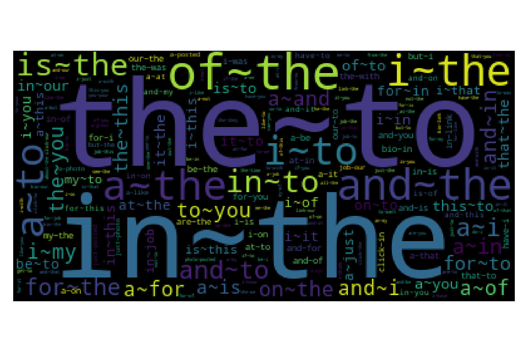
The following figure presents the word cloud of the difference. It can be observed that the main difference between the important bigrams of the former figure and this one is that the former presented mostly stopwords, and this one has other words.

Hypothesis Testing
We have been using the difference between \(\mathbb P(\mathcal X, \mathcal Y) - \mathbb P(\mathcal X) \mathbb P(\mathcal Y)\) to measure whether the variables are dependent or independent. For the case of rolling dices, we saw that when the variables are independent, all the absolute value of the difference is lower than \(0.009\); however, this is by no means a formal definition.
Hypothesis testing aims to measure whether the data collected agrees with a null hypothesis or can be discarted. For example, let us believe that the exposure of a particular substance is the cause of a deadly disease, then the following experiment can be created. On the one hand, there is a group that has been exposed to the substance, and on the other hand, the group has not been exposed. These two groups allow to accept or reject the null hypothesis that the substance is not related to the disease.
In the case at hand, hypothesis testing is helpful to state the dependency or independence of the random variables. One measures whether the estimated bivariate distribution supports the null hypothesis that the variables are independent, i.e., \(\mathcal H_0: \mathbb P(\mathcal X, \mathcal Y) - \mathbb P(\mathcal X) \mathbb P(\mathcal Y) = 0;\) where the alternative hypothesis is \(\mathcal H_1: \mathbb P(\mathcal X, \mathcal Y) - \mathbb P(\mathcal X) \mathbb P(\mathcal Y) \neq 0.\)
One can use different procedures in Hypothesis testing; selecting one of them depends on the characteristics of the random variables and the type of test. We will use two different tests for the problem we are dealing with: the Wald test and the other is Likelihood ratios.
The Wald Test
The Wald test is defined using the \(\hat \theta\) which is the estimation of \(\theta\) and \(\hat{\textsf{se}}\) the estimated standard error of \(\hat \theta\). The null and alternative hypothesis are \(\mathcal H_0: \hat \theta = \theta_0\) and \(\mathcal H_1: \hat \theta \neq \theta_0,\) respectively. Additionally, considering that \(\hat \theta\) is asymptotically normal, i.e., \(\frac{\hat \theta - \theta_0}{\hat{\textsf{se}}} \rightsquigarrow \mathcal N(0, 1),\) it can be defined that the size \(\alpha\) of the Wald test is rejecting \(\mathcal H_0\) when \(\mid W \mid > z_{\frac{\alpha}{2}}\) where
\[W = \frac{\hat \theta - \theta_0}{\hat{\textsf{se}}}.\]The relationship between \(\hat \theta\), \(\hat{\textsf{se}}\) and \(\theta_0\) with \(\mathbb P(\mathcal X, \mathcal Y)\) and \(\mathbb P(\mathcal X) \mathbb P(\mathcal Y)\) is the following. \(\theta_0\) defines the null hypothesis that in our case is that the variables are independent, i.e., \(\mathbb P(\mathcal X) \mathbb P(\mathcal Y).\) On the other hand, \(\mathbb P(\mathcal X, \mathcal Y)\) corresponds to \(\hat \theta\) and \(\hat{\textsf{se}}\) is the estimated standard error of \(\mathbb P(\mathcal X, \mathcal Y).\)
We can estimate the values for \(\hat \theta\) and \(\theta_0\), the only variable missing is \(\hat{\textsf{se}}\). The standard error is defined as \(\textsf{se} = \sqrt{V(\hat \theta)}\), in this case \(\theta = \mathbb P(\mathcal X_r, \mathcal X_c)\) is a bivariate distribution where the pair of random variables are drawn from a Categorical distribution with parameter \(\mathbf p\). The variance of a Categorical distribution is \(\mathbf p_i = \mathbf p_i (1 - \mathbf p_i),\) and the variance of \(\hat{\mathbf p_i}\) is \(\frac{\mathbf p_i (1 - \mathbf p_i)}{N};\) therefore, \(\hat{\textsf{se}} = \sqrt{\frac{\mathbf p_i (1 - \mathbf p_i)}{N}}.\)
For example, the Wald test for data collected on the two rolling dices example is computed as follows. Variable Z contains the drawn from two dices with the characteristic that \(\mathcal X_r=2\) with a probability \(0.1\) when \(\mathcal X_c=1.\) Variable \(W\) is the estimated bivariate distribution, i.e., \(\theta\), \(\hat{\textsf{se}}\) is identified using W as shown in the second line, and, finally, the third line has the Wald statistic.
N = len(Z)
se = np.sqrt(W * (1 - W) / N)
wald = (W - ind) / se
The Wald statistic is seen in the following matrix; the absolute value of the elements are compared against \(z_{\frac{\alpha}{2}}\) to accept or reject the null hypothesis. \(z_{\alpha}\) is the inverse of the standard normal distribution (i.e., \(\mathcal N(0, 1)\)) that gives the probability \(1-\alpha\), traditionally \(\alpha\) is \(0.1\) or \(0.05\). For a \(\alpha=0.01\) the value of \(z_{\frac{\alpha}{2}}\) is approximately \(2.58\) (variable c).
alpha = 0.01
c = norm.ppf(1 - alpha / 2)
Comparing the absolute values of W against \(2.58\), it is observed that \(\mathcal X_r=2\) and \(\mathcal X_c=1\) are dependent which corresponds to the designed of the experiment, the other pair that is found dependent is \(\mathcal X_r=4\) and \(\mathcal X_c=1.\)
The Wald test can also be applied to the bigrams example, as shown in the following code. The estimated bivariate distribution is found on variable co_occurrence; given that the matrix is sparse, the Wald statistic is only computed for those elements different than zero.
N = sum(list(bigrams.values()))
se = lambda x: np.sqrt(x * (1 - x) / N)
_ = [(bigram, [index[x] for x in bigram.split("~")])
     for bigram in bigrams]
co = co_occurrence
wald = {k: (co[i, j] - M[i] * M[j]) / se(co[i, j])
        for k, (i, j) in _}
Variable wald contains the statistic for all the bigrams, then we need to compare it against \(z_{\frac{\alpha}{2}}\); however, in the bigrams case, as mentioned previously, we are interested only on the bigrams that the probability of observing the pair is higher than the product of the marginals.
wald = {k: v for k, v in wald.items() if v > c}
It can be observed that variable wald has less than 10% of all the bigrams; unfortunately, these are still a lot and cannot be visualized in a table; consequently, we rely on the word cloud shown below.

As can be seen, the most important bigrams are similar to the ones observed on the difference figure; this is because the former approach and the Wald test are equivalent; the advantage of the Wald test is that there is a threshold that can be used to eliminate uninterested bigrams.
Likelihood ratios
The Wald test assumes normality on the estimation, which is a fair assumption when the number of counts is high; however, for the case of bigrams, as we have seen on the Vocabulary Laws, the majority of words appear infrequent; thus most of the bigrams are also infrequent.
The likelihood ratios are more appropriate for this problem; the idea is to model two hypotheses that encode the behavior of collocations. On the one hand, the first hypothesis is \(\mathcal H_1: \mathbb P(\mathcal X_c=w_2 \mid \mathcal X_r=w_1) = p = \mathbb P(\mathcal X_c=w_2 \mid \mathcal X_r=\neg w_1)\) which corresponds to the independence assumption. On the other hand, the second hypothesis is \(\mathcal H_2: \mathbb P(\mathcal X_c=w_2 \mid \mathcal X_r=w_1) = p_1 \neq p_2 = \mathbb P(\mathcal X_c=w_2 \mid \mathcal X_r=\neg w_1).\) Then the log of the likelihood ratio $\lambda$ is defined as follows:
\[\log \lambda = \log \frac{\mathcal L(\mathcal H_1)}{\mathcal L(\mathcal H_2)},\]where \(\mathcal L(\mathcal H_1)\) is the likelihood of observing the counts for words \(w_1\) and \(w_2\) and the bigram \((w_1, w_2)\) that corresponds to the hypothesis \(\mathcal H_1.\) Equivalent, \(\mathcal L(\mathcal H_2)\) corresponds to the likelihood of observing the counts for the second hypothesis.
Using \(c_1\), \(c_2\), and \(c_{12}\) for the count of the words \(w_1\) and \(w_2\) and the bigram \((w_1, w_2)\) the likelihood of the hypothesis are \(\mathcal L(\mathcal H_1)=L(c_{12}, c_1, p)L(c_2-c_{12}, N-c_1, p)\) and \(\mathcal L(\mathcal H_2)=L(c_{12}, c_1, p_1)L(c_2-c_{12}, N-c_1, p_2),\) where \(L(k, n, x) = x^k(1-x)^{n-k}.\)
The first step is to store the counts \(c_1\) and \(c_2\) on the variable count.
count = dict()
for k, v in bigrams.items():
    for x in k.split('~'):
        try:
            count[x] += v / 2
        except KeyError:
            count[x] = v / 2
The function \(L\) and the ratio can be computed as follows.
N = sum(list(count.values()))

def L(k, n, x):
    f1 = k * np.log(x)
    f2 = (n - k) * np.log(1 - x)
    return f1 + f2

def ratio(k):
    a, b = k.split('~')
    c12 = bigrams[k]
    c1 = count[a]
    c2 = count[b]
    p = c2 / N
    p1 = c12 / c1
    p2 = (c2 - c12) / (N - c1)
    f1 = L(c12, c1, p) +  L(c2 - c12, N - c1, p)
    f2 = L(c12, c1, p1) + L(c2 - c12, N - c1, p2)
    return -2 * (f1 - f2)
The last step is to obtain the statistic for each pair, and select only those bigrams where the null hypothesis (in this case \(\mathcal H_1\)) can be rejected.
r = {k: ratio(k) for k, v in bigrams.items()}
c = chi2.ppf((1 - alpha), 1)
r = {k: v for k, v in r.items() if np.isfinite(v) and v > c}
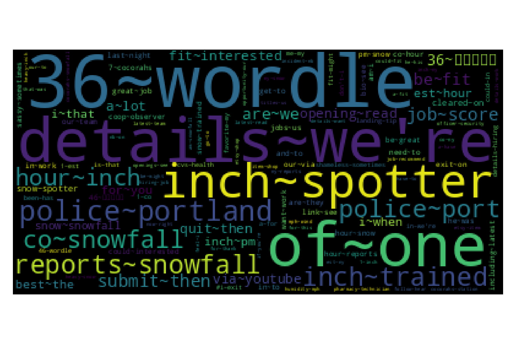
The following figure presents the word cloud obtained using the Likelihood method, and please take a minute to compare the three different word clouds produced so far.

Code of the Likelihood ratios word cloud
wc = WC().generate_from_frequencies(r)
plt.imshow(wc)
plt.axis('off')
plt.tight_layout()
Activities
As seen in the figures, the bigrams do not clearly indicate the events that occurred on the day, and few bigrams can be considered as a collocation. This behavior is normal; however, we can further analyze the test data to understand their behavior better.
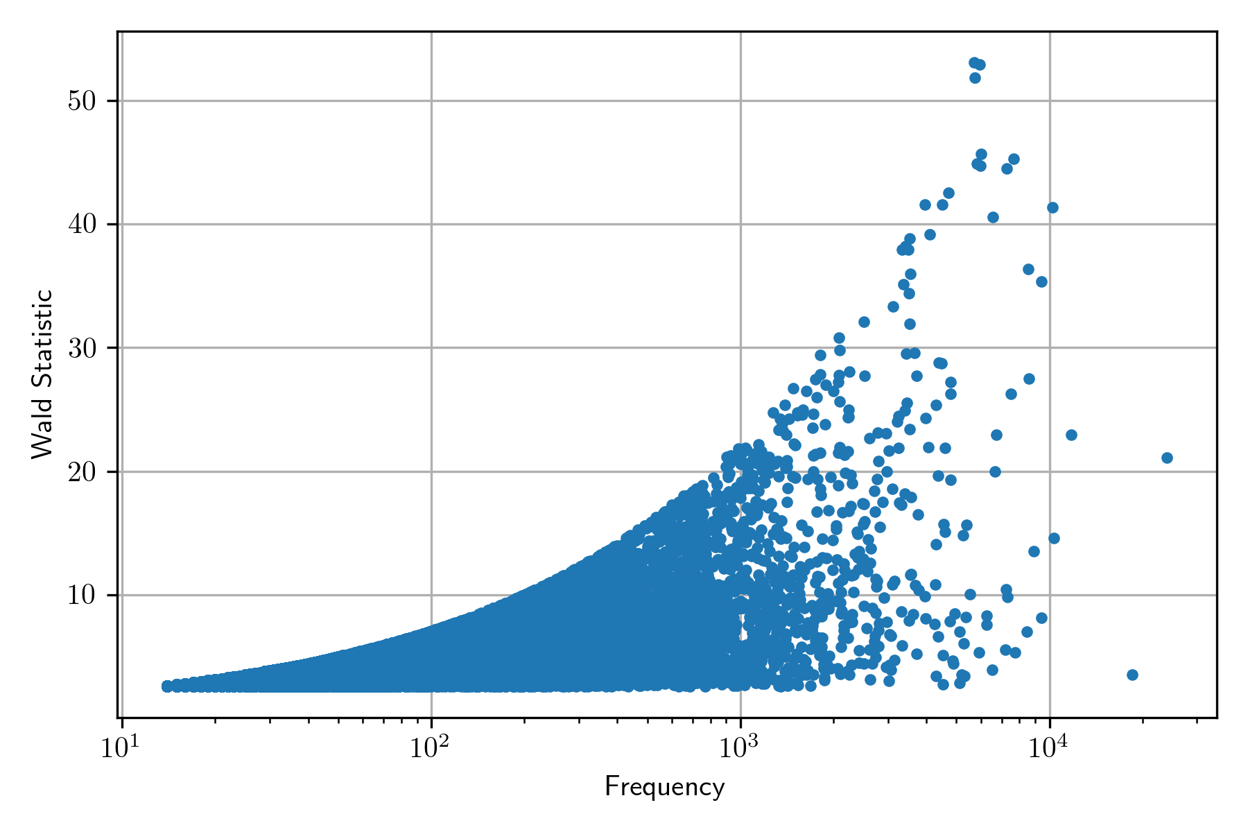
The following figure presents the scatter plot between frequency and Wald statistic. It can be observed that the Wald statistic increases when the frequency increases. This behavior is reflected in the word cloud; the result is that the bigrams appearing are the ones with higher frequency.
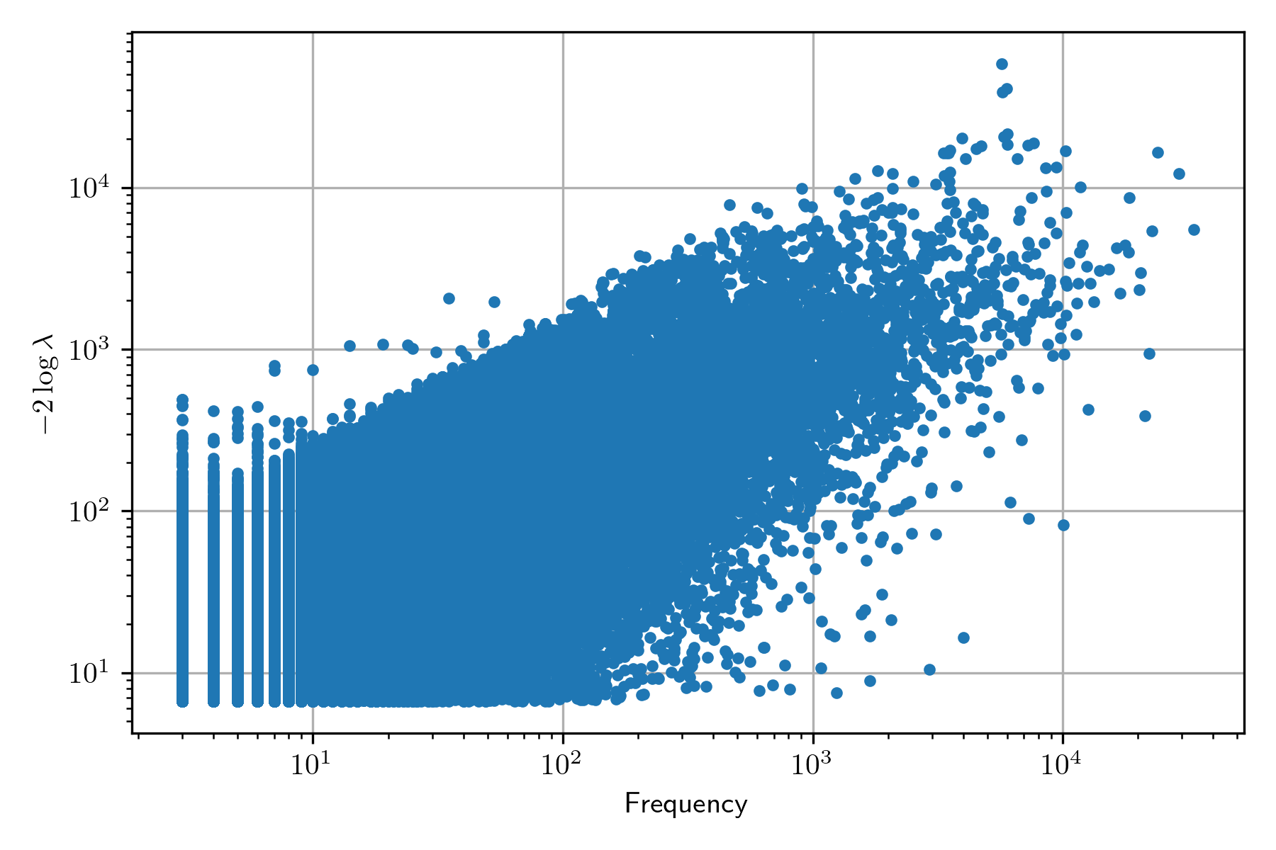
Conversely, the behavior of the Likelihood ratio does not present an increased value when the frequency is increased, as can be seen in the following figure; nonetheless, the word cloud is not as informative as one wishes to be.
So far, we have used the information of January 10, 2022; in this section, we will be working with January 17, 2022, to complement our analysis of finding collocations through hypothesis testing. The following figure presents the word cloud using the Likelihood test – it is essential to mention that it presents another limitation: it only contains 200 words corresponding to the words with higher values.

There are some similarities with the word cloud from the other day; however, there are significant differences. For example, it can be inferred that there was snow on that day and Martin Luther King memorial day. The word cloud of the following 200 words is shown below; it can be observed that the recurrent term is snow.